Bayesian vs Least Squares: A Modern Guide to Enzyme Kinetic Parameter Estimation for Biomedical Research

Abstract

Accurate estimation of enzyme kinetic parameters (e.g., Vmax, KM, Ki) is fundamental to understanding biological mechanisms, predicting drug interactions, and guiding therapeutic development. This article provides a comprehensive, comparative analysis of two core statistical frameworks: the traditional least-squares regression and the increasingly prominent Bayesian inference. Tailored for researchers and drug development professionals, the scope ranges from foundational philosophical and statistical principles to practical methodological implementation, troubleshooting of common pitfalls, and rigorous validation strategies. We synthesize recent methodological advances to offer clear guidance on selecting and optimizing the appropriate estimation approach based on data quality, prior knowledge, and the specific goals of the kinetic study, ultimately aiming to enhance the reliability and efficiency of biomedical research.

Core Philosophies in Enzyme Kinetics: Understanding Least Squares Assumptions and Bayesian Probability

In biochemical research and drug development, the quantification of kinetic parameters from experimental data is foundational for understanding enzyme behavior, metabolic pathways, and drug mechanisms. The Michaelis-Menten equation, which describes the relationship between substrate concentration and reaction rate via parameters Vmax and Km, is a cornerstone of this analysis [1]. However, experimental data is invariably contaminated by measurement noise—unwanted deviations arising from instrumentation, biological variability, and environmental fluctuations [2]. This noise transforms parameter estimation from a straightforward calculation into a central challenge in systems biology and pharmacokinetics [3].

The choice of estimation methodology critically determines how this noise is processed and interpreted, directly impacting the reliability of the resulting parameters. Traditional least squares regression methods, including linearized transformations like the Lineweaver-Burk and Eadie-Hofstee plots, have been widely used for their simplicity [1]. In contrast, Bayesian inference approaches explicitly model uncertainty by incorporating prior knowledge and providing probability distributions for parameter estimates [4]. This comparison guide objectively evaluates the performance of these paradigms in the face of noisy data, providing researchers with a clear framework for selecting estimation methods that yield accurate, precise, and trustworthy parameters for predictive modeling and decision-making [5].

Methodological Comparison: Protocols and Data Generation

A rigorous comparison of estimation methods requires standardized, reproducible experimental and computational protocols. The following sections detail the key methodologies for generating noisy biochemical data and the subsequent parameter estimation processes.

Experimental Protocol: Simulating Noisy Enzyme Kinetic Data

A robust protocol for comparing estimation methods begins with the generation of simulated kinetic data where the "true" parameter values are known, allowing for direct accuracy assessment [1].

• Step 1: Define True Kinetic Parameters. Based on a known enzyme system (e.g., invertase with Vmax = 0.76 mM/min and Km = 16.7 mM), define the error-free Michaelis-Menten relationship [1].
• Step 2: Generate Error-Free Time-Course Data. Using numerical integration (e.g., with the deSolve package in R), simulate substrate depletion over time for a set of initial substrate concentrations (e.g., 20.8, 41.6, 83, 166.7, 333 mM) [1].
• Step 3: Introduce Stochastic Noise. Corrupt the error-free data by adding random noise to create realistic "observed" data. Two primary error models are used:
  • Additive Error Model: [S]i = [S]pred + ε1i, where ε1 is a random variable from a normal distribution (mean=0, SD=0.04) [1].
  • Combined Error Model: [S]i = [S]pred + ε1i + [S]pred × ε2i, where ε2 is a random variable from a normal distribution (mean=0, SD=0.1). This model accounts for both fixed measurement noise and noise proportional to the signal magnitude [1].
• Step 4: Monte Carlo Replication. Repeat Step 3 to create a large number of replicate datasets (e.g., 1,000) for each error scenario. This ensemble approach allows for statistical analysis of estimator performance across many instances of random noise [1].

Parameter Estimation Protocols

From each noisy dataset, parameters are estimated using different methods. The workflow for preparing data and executing fits is critical for a fair comparison [1].

Data Preparation & Estimation Workflow

• Estimation Method 1 & 2: Linearization (LB, EH). Initial velocities (Vi) are calculated from the early linear phase of the substrate depletion curve for each concentration. For the Lineweaver-Burk (LB) method, the reciprocal data (1/Vi vs. 1/[S]) is fit with linear regression. For the Eadie-Hofstee (EH) method, Vi is plotted against Vi/[S] and fit linearly [1].
• Estimation Method 3 & 4: Direct Nonlinear Regression (NL, ND). The Michaelis-Menten equation is fit directly to velocity-substrate data using nonlinear least squares. The NL method uses the initial velocity (Vi). The ND method uses the average velocity (VND) calculated between adjacent time points and the corresponding average substrate concentration ([S]ND) [1].
• Estimation Method 5: Nonlinear Regression of Time-Course Data (NM). This most advanced method fits the integrated form of the Michaelis-Menten ordinary differential equation (ODE) directly to the full time-series substrate concentration data, without the need for preliminary velocity calculation [1].
• Bayesian Estimation Protocol. In a separate framework, prior distributions (e.g., log-normal) are defined for Vmax and Km based on existing literature or biological plausibility. Using computational tools (e.g., Markov Chain Monte Carlo sampling), the posterior distribution of the parameters is estimated, given the observed noisy data. This yields not just point estimates but full probability densities, quantifying uncertainty directly [4] [5].

Comparative Performance Analysis

The core of this guide is an objective comparison of how different estimation methods perform under controlled noisy conditions. The following tables summarize key quantitative findings from simulation studies.

Table 1: Performance of Estimation Methods with Different Error Types [1]

Estimation Method	Error Model	Relative Accuracy (Median % Bias)	Relative Precision (90% CI Width)	Key Characteristics
Lineweaver-Burk (LB)	Additive	High Bias (e.g., >15%)	Low Precision (Widest CI)	Linearizes data, distorts error structure.
Eadie-Hofstee (EH)	Additive	Moderate Bias	Moderate Precision	Less distortion than LB but still problematic.
Nonlinear (NL)	Additive	Low Bias	Good Precision	Direct fit, handles additive noise well.
Nonlinear (ND)	Additive	Low Bias	Good Precision	Uses more data points than NL.
Nonlinear (NM)	Additive	Lowest Bias	Best Precision	Uses all time-course data; most efficient.
Lineweaver-Burk (LB)	Combined	Very High Bias	Very Low Precision	Performs poorly with proportional error.
Nonlinear (NM)	Combined	Low Bias	Best Precision	Robust to complex error models.

Table 2: Bayesian vs. Least Squares in Data-Limited Scenarios [4]

Feature	Weighted Least Squares (Standard NL)	Bayesian Estimation	Subset-Selection Method
Core Philosophy	Find parameters minimizing sum of squared errors.	Update prior belief with data to obtain posterior distribution.	Fix inestimable parameters at prior values; estimate only key subset.
Handling Limited Data	Prone to overfitting; unreliable estimates.	Incorporates prior knowledge to stabilize estimates.	Reduces degrees of freedom to avoid overfitting.
Output	Point estimates & confidence intervals.	Full probability distributions (quantifies uncertainty).	Point estimates for a subset of parameters.
Reliance on Initial Guess	Moderate. Can converge to local minima.	High. Overly confident poor priors mislead.	Low. Less susceptible to poor initial guesses.
Computational Cost	Low to Moderate.	High (MCMC sampling).	Very High (requires estimability analysis).
Best Use Case	Abundant, high-quality data.	Prior knowledge is reliable and informative.	Model is large; prior knowledge is vague.

The Scientist's Toolkit: Essential Research Reagent Solutions

Selecting the right computational and analytical tools is as critical as choosing the right biochemical reagents. This table details key solutions for performing robust uncertainty quantification in enzyme kinetics.

Table 3: Research Reagent Solutions for Uncertainty Quantification

Item	Function in Estimation	Example/Platform	Relevance to Noise Challenge
NONMEM	Industry-standard software for nonlinear mixed-effects modeling. Used for advanced NM and NL methods [1].	NONMEM (ICON plc)	Directly models complex error structures (additive, proportional, combined) in time-course data.
R with deSolve & nls	Open-source environment for simulation (ODE integration) and nonlinear least-squares fitting [1].	R Statistical Language	Provides flexible framework for Monte Carlo simulation and custom estimator implementation.
Bayesian Inference Engine	Software for performing MCMC sampling to obtain posterior parameter distributions.	Stan, PyMC, JAGS	Quantifies parameter uncertainty directly and incorporates prior knowledge to combat noise [4] [5].
Global Optimizer	Solver to find best-fit parameters in complex, multi-modal landscapes common in nonlinear models.	MEIGO, SciPy optimize	Avoids convergence to local minima, ensuring more accurate point estimates from noisy data [5].
Graph Neural Network (GNN)	Machine learning architecture for predicting molecular properties with inherent uncertainty quantification [6].	Chemprop (D-MPNN)	Offers scalable UQ for high-dimensional design spaces (e.g., drug discovery), where noise is prevalent.
Conformal Prediction Toolkit	Framework for generating prediction sets with guaranteed coverage probabilities, regardless of data distribution.	crepes (Python)	Provides distribution-free, rigorous uncertainty intervals for model predictions in the presence of noise [7].

Discussion: Implications for Research and Development

The comparative data leads to a clear conclusion: nonlinear regression methods, particularly those leveraging full time-course data (NM) or Bayesian inference, provide superior accuracy and precision in the presence of experimental noise compared to traditional linearization techniques [1]. The Least Squares (LB, EH) methods fail because their required data transformations distort the inherent noise structure, violating the fundamental assumptions of linear regression and producing biased estimates [1].

The choice between advanced least squares (e.g., NM) and Bayesian methods hinges on the data context and the research goal. When data is plentiful and the primary need is a classic point estimate, nonlinear least squares (NM) is robust and efficient. However, in the prevalent real-world scenario of sparse, noisy data—common in early drug discovery or patient-specific modeling—Bayesian estimation becomes indispensable [4]. It formally integrates prior knowledge, provides a complete picture of parameter uncertainty, and can prevent overfitting. This is critical for building trust in automated, high-throughput experimentation platforms where UQ must be a built-in feature [8].

Philosophical Divergence in Handling Noise

Emerging trends point toward hybrid frameworks that combine mechanistic models (like Michaelis-Menten ODEs) with machine learning surrogates to manage uncertainty in highly complex systems [3]. Furthermore, techniques like conformal prediction are rising to provide strict, distribution-free guarantees on prediction intervals, offering a new layer of reliability for AI-driven discovery in biochemistry [7]. For the practicing scientist, the imperative is to move beyond simplistic linearization. Embracing nonlinear regression as a baseline and adopting Bayesian or other advanced UQ methods for challenging data scenarios will lead to more reproducible, reliable, and actionable biochemical insights.

Classical Least Squares (CLS), also known as Ordinary Least Squares (OLS), is a foundational parameter estimation method that minimizes the sum of squared differences between observed and predicted values [9]. In enzyme kinetics and drug development, accurate parameter estimation for models like the Michaelis-Menten equation is critical for predicting biological activity and drug interactions [10]. This guide compares the performance of Classical Least Squares against modern Bayesian alternatives within enzyme parameter estimation research, highlighting foundational principles, practical pitfalls, and data-driven performance metrics [4] [11].

Methodological Foundations: CLS vs. Bayesian Estimation

The core distinction between CLS and Bayesian methods lies in their philosophical approach to uncertainty and incorporation of prior knowledge.

• Classical Least Squares (CLS) is a deterministic, frequentist approach. It seeks a single set of parameter values that minimize the sum of squared residuals, providing point estimates [9]. Its validity depends on strict statistical assumptions, including linearity, homoscedasticity (constant error variance), and independence of errors [12] [13]. Violations of these assumptions can lead to biased and unreliable estimates.

• Bayesian Estimation is a probabilistic framework. It treats model parameters as random variables with distributions. The method combines prior knowledge (encoded as prior probability distributions) with experimental data (via the likelihood function) to form a posterior probability distribution for the parameters [4]. This directly quantifies estimation uncertainty and allows for the integration of diverse information sources.

The following diagram illustrates the fundamental logical and procedural differences between these two pathways for parameter estimation.

Quantitative Performance Comparison

The choice between CLS and Bayesian methods has tangible impacts on estimation accuracy, robustness, and experimental efficiency.

Foundational Comparison of Methodologies

The table below summarizes the core characteristics of each approach.

Table: Foundational Comparison of CLS and Bayesian Estimation Methods

Aspect	Classical Least Squares (CLS)	Bayesian Estimation
Core Philosophy	Frequentist; deterministic point estimation.	Probabilistic; parameters as distributions.
Use of Prior Knowledge	Not incorporated formally.	Explicitly incorporated via prior distributions.
Handling of Limited Data	Prone to overfitting and unreliable estimates [4].	Prior information stabilizes estimates, mitigating overfitting [4].
Output	Point estimates and approximate confidence intervals.	Full posterior distributions (mean, median, credible intervals).
Uncertainty Quantification	Indirect (e.g., confidence intervals).	Direct and inherent to the posterior distribution.
Computational Demand	Typically low; analytical or simple numerical solutions.	Can be high; often requires Markov Chain Monte Carlo (MCMC) sampling.
Robustness to Poor Initial Guesses	Can converge to local minima, sensitive to initialization.	More robust if priors are not overly confident and incorrect [4].

Performance in Enzyme Parameter Estimation

Recent studies directly comparing these paradigms reveal significant differences in performance, particularly with complex or limited data.

Table: Performance in Enzyme Kinetics & Drug Discovery Applications

Study Focus	CLS Performance & Limitations	Bayesian/Hybrid Performance	Key Supporting Data
Estimating Inhibition Constants (Ki) [10]	Conventional design requires data at multiple substrate/inhibitor concentrations. Prone to bias if model is misspecified.	50-BOA (IC50-Based Optimal Approach), integrating Bayesian-like prior structural knowledge, achieved accurate estimation with >75% fewer experiments using a single inhibitor concentration.	50-BOA reduced required data points by over 75% while maintaining precision [10].
Progress Curve Analysis [14]	Analytical integral methods require precise initial guesses and can be unstable. Direct OLS fitting of differential equations is sensitive to noise.	Numerical approaches using spline interpolation (akin to flexible Bayesian modeling) showed lower dependence on initial guesses and comparable/better accuracy.	Spline-based methods provided robust parameter estimates independent of initial values [14].
Enzyme Activity with GFET Data [11]	Standard nonlinear regression (e.g., CLS) to Michaelis-Menten models may fail with noisy, complex sensor data.	A hybrid Bayesian inversion-supervised learning framework outperformed standard methods in accuracy and robustness for estimating turnover number and Km.	The hybrid framework provided more accurate and robust predictions of enzyme behavior under varying conditions [11].
Drug Discovery Screening [15]	Not directly applicable to sequential experimental design.	Multifidelity Bayesian Optimization (MF-BO) efficiently integrated low (docking), medium (single-point), and high (dose-response) fidelity assays.	MF-BO discovered top-performing histone deacetylase inhibitors with sub-micromolar potency using significantly fewer high-cost experiments [15].

Experimental Protocols & Linearization Pitfalls

Canonical vs. Optimized Protocol for Enzyme Inhibition

A key area where methodology impacts practice is in estimating enzyme inhibition constants (K_ic, K_iu), vital for predicting drug-drug interactions [10].

A. Canonical CLS-Based Protocol:

• Determine IC50: Measure percentage control activity across a range of inhibitor concentrations at a single substrate concentration (often ~Km) [10].
• Design Experiment: Measure initial reaction velocities (V0) across a matrix of substrate concentrations (e.g., 0.2Km, Km, 5Km) and inhibitor concentrations (0, 1/3IC50, IC50, 3IC50) [10].
• Model Fitting: Use nonlinear least squares (an extension of CLS) to fit the mixed inhibition velocity equation (Equation 1 in [10]) to the dataset, minimizing the sum of squared residuals between observed and predicted V0.

B. Optimized 50-BOA Protocol (Informs Bayesian Design):

• Determine IC50: As in the canonical protocol.
• Design Experiment: Perform kinetics experiments using only a single inhibitor concentration (I_T) greater than the IC50, across a range of substrate concentrations [10].
• Constrained Fitting: Fit the same kinetic model, but incorporate the known harmonic mean relationship between IC50 and the inhibition constants as a structural prior. This reduces the effective parameter space and allows precise estimation from minimal data [10].

The Pitfall of Linearization in CLS

To enable the use of simple linear least squares, enzyme kinetic models like the Michaelis-Menten equation are often linearized (e.g., Lineweaver-Burk plot). This practice introduces significant pitfalls:

• Error Distortion: Linearization transforms the error structure of the data. Errors that are normally distributed in the original V0 measurements become heteroscedastic (non-constant variance) in the transformed space, violating a core OLS assumption [13]. This gives unequal weight to data points, yielding biased estimates.
• Amplification of Noise: Data points at low substrate concentrations (high values in a Lineweaver-Burk plot) become disproportionately influential, amplifying experimental noise and leading to inaccurate parameter estimates.

Modern practice strongly favors direct nonlinear least squares fitting to the original, untransformed model, which preserves the correct error structure, though it requires iterative numerical methods.

Critical Error Assumptions of CLS and Their Violations

The reliability of CLS estimates hinges on several statistical assumptions, the violation of which is common in biochemical data [12] [13].

Table: Key OLS Assumptions and Consequences of Violation in Enzyme Kinetics

OLS Assumption	Meaning	Common Violation in Kinetic Studies	Consequence & Mitigation
Linearity in Parameters	The model must be a linear function of the parameters being estimated.	Enzyme kinetic models (e.g., V_max, K_m) are inherently nonlinear.	Use nonlinear least squares. Linearizing transforms (e.g., Lineweaver-Burk) violate other assumptions.
Homoscedasticity	Constant variance of errors across all observations.	Errors in velocity measurements often increase with the magnitude of V0.	Use weighted least squares, where each data point is weighted inversely to its variance. Model the error structure explicitly in Bayesian frameworks.
Independence of Errors	No correlation between residual errors.	Progress curve data, where sequential measurements come from the same reaction mixture, show autocorrelation [14].	Use techniques designed for time-series data (e.g., modeling error covariance) or use progress curve analysis methods [14].
Normality of Errors	Residuals should be normally distributed.	Outliers from experimental artifacts or model misspecification can create heavy-tailed error distributions.	Robust regression techniques or Bayesian methods with t-distributed error models offer more resilience.

The following workflow diagram for the optimized 50-BOA protocol illustrates how a smarter experimental design, informed by error landscape analysis, can overcome some limitations of traditional CLS approaches.

The Scientist's Toolkit: Research Reagent Solutions

Table: Essential Reagents & Materials for Enzyme Parameter Estimation Studies

Item	Typical Function in Experiment	Consideration for Estimation
Purified Enzyme	The biocatalyst of interest. Source, purity, and specific activity must be standardized and reported.	Batch-to-batch variability can be modeled as a random effect in hierarchical Bayesian models.
Substrate(s)	The molecule(s) transformed by the enzyme. Should be >99% purity.	Stock concentration accuracy is critical. Errors propagate into parameter estimates.
Inhibitor(s)	Compound(s) used to probe enzyme function and mechanism.	Solubility and stability in assay buffer are key. DMSO concentrations must be controlled.
Detection System	Method to quantify reaction progress (e.g., fluorescence plate reader, HPLC, GFET sensor [11]).	Defines the noise characteristics (error variance) of the V0 data, impacting weighting in CLS or likelihood in Bayesian.
Assay Buffer	Provides optimal pH, ionic strength, and cofactors for enzyme activity.	Conditions must ensure stable activity throughout the measurement period to avoid confounding trends.
Positive/Negative Controls	Validates assay performance (e.g., no-enzyme control, known inhibitor control).	Essential for defining 0% and 100% activity baselines for robust IC50 determination [10].
Software	For analysis (e.g., R, Python, GraphPad Prism, MATLAB, custom Bayesian MCMC tools like Stan).	Choice determines accessibility to advanced methods like Bayesian estimation or spline-based progress curve analysis [14].

Classical Least Squares provides a transparent, computationally simple foundation for parameter estimation but is constrained by its strict assumptions and lack of a formal mechanism to incorporate prior knowledge or fully quantify uncertainty. In contrast, Bayesian methods and modern hybrid approaches offer a powerful, probabilistic framework that is particularly advantageous for complex enzyme kinetic studies with limited or noisy data, as prevalent in drug development.

The evidence indicates that Bayesian methods are often preferred when reliable prior knowledge exists, as they provide robust, information-rich estimates and can dramatically reduce experimental burden through optimal design [4] [10]. However, CLS and nonlinear least squares remain vital tools, especially for initial exploratory analysis, when priors are weak or unreliable, or when computational simplicity is paramount. The evolving best practice lies in selecting the tool based on the problem context: using CLS for well-behaved systems with abundant data, and leveraging Bayesian strategies for high-stakes estimation, complex models, or when maximizing information from every experiment is critical.

The transition from traditional least squares estimation to Bayesian methods represents a fundamental paradigm shift in enzyme parameter estimation and metabolic engineering. While classical approaches yield single-point parameter estimates, Bayesian inference provides complete probabilistic distributions that quantify uncertainty—a critical advancement for drug development and bioproduction where experimental data is inherently noisy and limited. This comparison guide objectively evaluates these competing methodologies within the broader thesis that Bayesian frameworks offer superior uncertainty quantification and information integration for complex biological systems, albeit with increased computational demands. Recent research demonstrates how Bayesian methods like BayesianSSA integrate environmental information from perturbation data to improve predictions in metabolic networks [16], while least squares approaches combined with model reduction techniques remain valuable for well-posed parameter estimation problems with complete data [17].

Methodological Comparison: Foundational Principles

Least squares minimization operates on frequentist principles, seeking parameter values that minimize the sum of squared differences between model predictions and observed data. This approach yields deterministic point estimates with confidence intervals derived from asymptotic approximations. In contrast, Bayesian updating treats parameters as random variables with probability distributions [18]. Beginning with prior distributions representing initial beliefs, Bayesian methods update these to posterior distributions via Bayes' theorem, incorporating experimental evidence through likelihood functions. This probabilistic framework naturally quantifies parameter uncertainty and facilitates the integration of diverse data types.

The computational implications are significant: least squares optimization typically requires less computational effort, while Bayesian approaches employing Markov Chain Monte Carlo (MCMC) methods like the Metropolis-Hastings algorithm demand substantially more resources to approximate posterior distributions [18]. However, this computational investment yields richer inference, capturing multi-modal distributions and parameter correlations often missed by point-estimate methods.

Quantitative Performance Comparison

The practical performance differences between these methodologies are evident across multiple metrics relevant to researchers and drug development professionals.

Table 1: Methodological Comparison of Parameter Estimation Approaches

Characteristic	Least Squares Minimization	Bayesian Inference	Practical Implications
Parameter Output	Point estimates with approximate confidence intervals	Full posterior probability distributions	Bayesian posteriors enable direct probability statements about parameters
Uncertainty Quantification	Based on curvature of objective function at optimum	Intrinsic to posterior distribution	Bayesian approach captures asymmetric and multi-modal uncertainties
Prior Information Integration	Challenging to incorporate formally	Natural framework through prior distributions	Bayesian methods leverage historical data or biological constraints [16]
Computational Demand	Generally lower (optimization problem)	Higher (MCMC sampling or variational inference) [18]	Least squares preferable for very large models with complete data
Identifiability Assessment	Local evaluation via Hessian matrix	Global evaluation via posterior inspection	Bayesian methods reveal parameter correlations and non-identifiabilities
Required Parameters per Reaction	Varies with kinetic model (e.g., 2 for Michaelis-Menten)	Often fewer (e.g., BayesianSSA requires 1 for one-substrate reaction) [16]	Bayesian methods can reduce parameterization burden

Table 2: Experimental Performance in Case Studies

Study/Application	Method	Performance Metric	Result	Key Insight
E. coli Central Metabolism Prediction [16]	BayesianSSA	Prediction accuracy for perturbation responses	Successfully integrated environmental data into structural predictions	Bayesian approach reduced indefinite predictions from SSA
Trypanosoma brucei Trypanothione Synthetase [17]	Weighted Least Squares	Training error	0.70	Least squares effective with complete concentration data
Trypanosoma brucei Trypanothione Synthetase [17]	Unweighted Least Squares	Training error	0.82	Weighting improved fit for this system
Nicotinic Acetylcholine Receptors [17]	Weighted Least Squares	Training error	3.61	Higher error suggests model mismatch or noisy data
Metabolic Engineering Optimization [19]	Bayesian Optimization	Convergence to optimum	22% of experimental points vs. grid search	Dramatic reduction in experimental resources required
Progress Curve Analysis [14]	Spline-based Numerical Approach	Dependence on initial estimates	Lower than direct integration methods	Hybrid approaches can mitigate initialization sensitivity

Experimental Protocols and Workflows

Objective: Predict metabolic flux responses to enzyme perturbations by integrating structural network information with environmental data.

Protocol:

• Network Structural Encoding: Represent the metabolic network as a stoichiometric matrix (ν) where rows correspond to metabolites and columns to reactions.
• SSA Variable Definition: Define matrix R(r) with elements rj,m = ∂Fj/∂x_m representing reaction sensitivities to metabolite concentrations.
• Prior Distribution Specification: Assign prior distributions to SSA variables based on general biological knowledge or historical data.
• Perturbation Data Integration: Collect perturbation-response datasets from the target environment and compute likelihood functions.
• Posterior Estimation: Use MCMC sampling to obtain posterior distributions for SSA variables given perturbation data.
• Response Prediction: Calculate posterior predictive distributions for flux changes to novel perturbations using the updated SSA variables.
• Validation: Compare predictions against hold-out experimental data or synthetic benchmarks.

Key Advantage: This Bayesian approach reduces indefinite predictions from structural analysis alone by incorporating environmental-specific data.

Objective: Estimate kinetic parameters when only partial concentration measurements are available.

Protocol:

• Model Reduction: Apply Kron reduction to the original kinetic model to eliminate unmeasured species, creating a reduced model governed by the same kinetic law (e.g., mass action).
• Parameter Transformation: Express reduced model parameters as functions of original model parameters.
• Preliminary Estimation: Use weighted or unweighted least squares to fit the reduced model to available time-series concentration data.
• Error Metric Definition: Introduce a trajectory-independent measure quantifying dynamical differences between original and reduced models.
• Original Parameter Estimation: Solve an optimization problem minimizing the difference measure to estimate original model parameters.
• Cross-Validation: Apply leave-one-out cross-validation to determine whether weighted or unweighted least squares is preferable for the specific system.
• Identifiability Check: Assess whether parameters are uniquely determinable from the available measurements.

Key Advantage: Transforms ill-posed estimation problems with incomplete data into well-posed problems through model reduction.

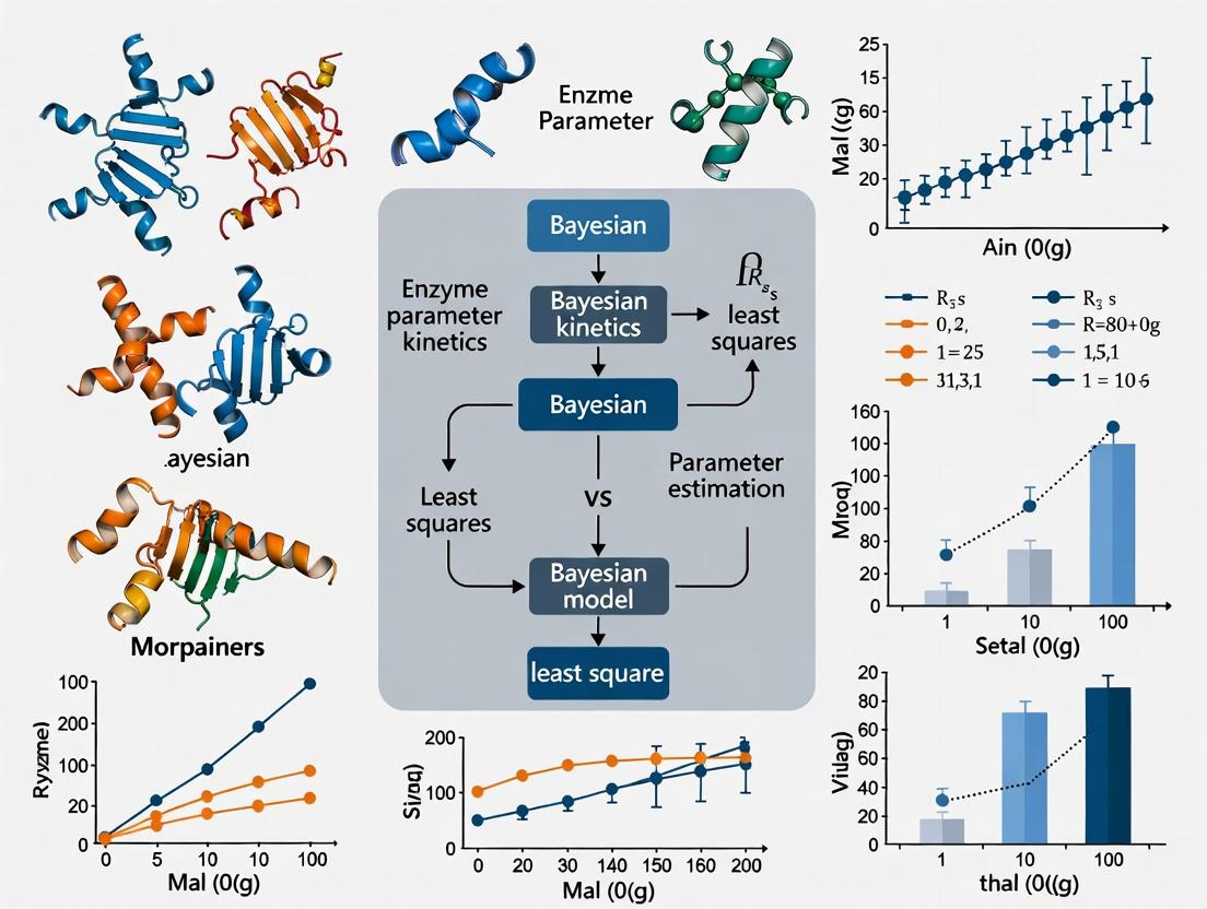
Bayesian vs Least Squares Workflow Comparison

Applications in Drug Development and Metabolic Engineering

Model-Based Design of Experiments (MBDoE): Bayesian approaches significantly enhance MBDoE for parameter precision in enzyme kinetic characterization [20]. By quantifying parameter uncertainty through posterior distributions, researchers can design experiments that maximize information gain about uncertain parameters. This is particularly valuable in drug development where experimental resources are limited and each data point is costly to obtain. Recent advances in MBDoE address challenges in real industrial scenarios, improving robustness and reliability of model calibration [20].

Progress Curve Analysis: Traditional initial slope analysis for enzymatic reactions requires substantial experimental effort. Progress curve analysis offers efficient alternatives, with Bayesian methods providing natural frameworks for handling measurement noise and parameter correlations [14]. Comparative studies show that spline-based numerical approaches exhibit lower dependence on initial parameter estimates compared to direct integration methods, though analytical approaches remain limited in applicability [14].

Bayesian Optimization of Bioproduction: In synthetic biology and metabolic engineering, Bayesian optimization has emerged as a powerful strategy for optimizing complex enzymatic pathways with minimal experimental iterations [19]. The Imperial iGEM 2025 team's BioKernel framework demonstrates how Bayesian optimization can identify optimal induction conditions for multi-enzyme pathways using dramatically fewer experiments than grid search approaches—converging to optima in approximately 22% of the experimental points required by traditional methods [19].

BayesianSSA Integration of Structural and Environmental Information

Table 3: Research Reagent Solutions for Enzyme Parameter Estimation

Tool/Reagent	Function	Method Compatibility	Key Considerations
Perturbation Datasets	Provide response data for enzyme activity changes	BayesianSSA, Validation for both methods	Quality and relevance to target environment critical [16]
Kinetic Model Software	Implement differential equation models of enzyme systems	Both (different implementations)	MATLAB libraries available for Kron reduction approaches [17]
MCMC Sampling Algorithms	Generate samples from posterior distributions	Bayesian methods exclusively	Metropolis-Hastings common but computationally intensive [18]
Progress Curve Analysis Tools	Extract kinetic parameters from time-course data	Both (different statistical frameworks)	Spline-based methods reduce initial value sensitivity [14]
Model-Based DoE Platforms	Design optimal experiments for parameter estimation	Bayesian methods particularly benefit	Maximizes information gain from limited experiments [20]
Bayesian Optimization Frameworks	Optimize multi-parameter biological systems	Bayesian methods exclusively	BioKernel offers no-code interface for biologists [19]
Structural Network Databases	Provide stoichiometric matrices for metabolic networks	BayesianSSA, Structural analysis	Kyoto Encyclopedia of Genes and Genomes (KEGG) commonly used

Decision Framework and Future Perspectives

The choice between Bayesian and least squares methodologies depends on multiple factors including data completeness, computational resources, and uncertainty quantification needs. For well-posed problems with complete concentration measurements and limited computational resources, least squares approaches combined with model reduction techniques offer practical solutions [17]. When facing indefinite predictions from structural models, partial or noisy data, or requirements for comprehensive uncertainty quantification, Bayesian methods provide superior frameworks [16] [18].

Future developments in enzyme parameter estimation will likely focus on hybrid approaches that leverage strengths of both paradigms. Promising directions include approximate Bayesian computation methods that reduce computational burdens, and sequential experimental design frameworks that integrate MBDoE with real-time Bayesian updating. The increasing availability of high-throughput experimental data from automated platforms will further drive adoption of Bayesian methods that can effectively integrate diverse data types while quantifying uncertainties essential for robust decision-making in drug development.

Decision Framework for Method Selection

Conceptual Foundations: A Comparative Framework

The choice between frequentist and Bayesian statistical paradigms fundamentally shapes how scientists approach parameter estimation, interpret results, and quantify uncertainty. This section delineates the core conceptual components and their practical implications for research.

Core Definitions and Philosophical Contrast

The distinction between the frameworks begins with their definition of probability. The frequentist approach interprets probability as the long-term frequency of an event occurring in repeated identical trials [21]. Parameters (e.g., the true Michaelis constant, Km) are considered fixed but unknown quantities. In contrast, the Bayesian framework views probability as a degree of belief or confidence in an event [21]. Parameters are treated as random variables described by probability distributions, allowing researchers to make direct probabilistic statements about them [21].

The process of learning from data differs accordingly. A frequentist uses the likelihood—the probability of observing the collected data given a specific parameter value—to find the most probable parameter value that explains the evidence, a method known as maximum likelihood estimation (MLE) [22]. The Bayesian approach formalizes learning by starting with a prior distribution, which encapsulates existing knowledge or belief about a parameter before seeing the new data. This prior is then updated with the likelihood of the observed data via Bayes' theorem to yield the posterior distribution [22] [23]. The posterior represents a complete synthesis of old and new information, containing all current knowledge about the parameter [23]. The foundational Bayes' formula is: Posterior ∝ Likelihood × Prior [23].

Table 1: Foundational Comparison of Frequentist and Bayesian Approaches

Aspect	Frequentist Approach	Bayesian Approach
Nature of Parameters	Fixed, unknown constants [21].	Random variables with probability distributions [21].
Core Objective	Estimate fixed parameter values (e.g., via MLE) and construct frequency-based intervals [22].	Derive the posterior probability distribution of parameters [23].
Use of Prior Information	Not formally incorporated.	Formally incorporated via the prior distribution [22].
Interpretation of Uncertainty	Expressed as confidence intervals, based on hypothetical repeated sampling [24].	Expressed as credible intervals, derived directly from the posterior distribution [24].
Typical Output	Point estimate (e.g., MLE) and a confidence interval [25].	Entire posterior distribution, summarized by a point estimate (e.g., mean) and a credible interval [23].

Illustrative Case Study: Diagnostic Testing

A classic example highlights the practical impact of these philosophical differences [22]. Consider a rare disease with a 0.1% prevalence (prior) and a diagnostic test that is 99% accurate (likelihood). A patient tests positive.

• A frequentist (maximum likelihood) analysis focuses solely on the test accuracy. Since the likelihood of a positive result given the disease (99%) is much higher than the likelihood of a positive result without the disease (1%), one might conclude a high probability of illness [22].
• A Bayesian analysis incorporates the low disease prevalence (prior) via Bayes' rule. The calculation shows the posterior probability of having the disease given a positive test is only about 9%, with a 91% probability of being healthy [22]. This counterintuitive result demonstrates how strong prior information can drastically alter conclusions drawn from data alone.

Uncertainty Quantification: Confidence vs. Credible Intervals

Both paradigms provide interval estimates to quantify uncertainty, but their interpretations are profoundly different and often confused [21].

A 95% Confidence Interval (CI) is a frequentist construct. Its correct interpretation is: "If we were to repeat the experiment an infinite number of times, 95% of the calculated CIs would contain the true, fixed population parameter" [21] [24]. It is a statement about the long-run performance of the method, not about the probability of the parameter lying in a specific observed interval. The parameter is fixed; the interval is random [21].

A 95% Credible Interval (CrI), also called a Bayesian confidence interval, is derived directly from the posterior distribution [24]. Its interpretation is more intuitive: "Given the observed data and the prior, there is a 95% probability that the true parameter value lies within this specific interval" [24]. Here, the parameter is random (described by a distribution), and the interval is fixed for a given posterior.

Table 2: Comparison of Confidence and Credible Intervals

Feature	95% Confidence Interval (Frequentist)	95% Credible Interval (Bayesian)
Philosophical Basis	Long-run frequency of the interval containing the fixed true parameter [21].	Degree of belief from the posterior distribution [24].
Interpretation of a Specific Interval	Incorrect: "There's a 95% chance the parameter is in this interval." Correct: "95% of such intervals from repeated experiments contain the parameter." [24]	Correct: "There is a 95% probability the parameter is in this interval." [24]
Incorporates Prior Knowledge?	No.	Yes, via the prior distribution.
Construction	Based on sampling distribution of the estimator (e.g., mean).	Derived from quantiles of the posterior probability distribution.
Width Influenced By	Sample size, data variability [24].	Sample size, data variability, and prior information.

Diagram 1: Contrasting Paths to Confidence and Credible Intervals (Max Width: 760px)

Application in Enzyme Kinetics: Bayesian vs. Least Squares Estimation

Estimating parameters like the maximum reaction rate (Vmax) and Michaelis constant (Km) from enzyme kinetic data (e.g., from spectrophotometric assays measuring initial velocity vs. substrate concentration) is a central task in biochemical research and drug discovery. The choice of estimation method significantly impacts the reliability and interpretability of these parameters.

Methodological Comparison

Nonlinear Least Squares (NLLS) is the standard frequentist approach. It finds parameter values that minimize the sum of squared residuals between observed reaction velocities and those predicted by a model (e.g., Michaelis-Menten). It yields a single best-fit parameter set with confidence intervals typically derived from linear approximations, which can be unreliable for nonlinear models with limited data [25].

Bayesian Parameter Estimation treats the parameters (Vmax, Km) as distributions. It starts with priors (e.g., Km must be positive, within a physiologically plausible range), uses the likelihood of the observed kinetic data, and computes a posterior distribution for the parameters [26]. This method naturally handles parameter uncertainty, correlations, and allows for direct probability statements (e.g., "There is a 90% probability that Km is between 2.1 and 3.0 mM").

Supporting Experimental Data and Protocol

A study applying Adaptive Population Monte Carlo Approximate Bayesian Computation (APMC) to estimate parameters of the Farquhar photosynthetic enzyme model provides a relevant experimental template for enzyme kinetics [26].

1. Experimental Protocol:

• Data Collection: Gather paired observational data. In the photosynthesis study, this was net CO₂ assimilation rate (A) vs. intercellular CO₂ concentration (Ci) [26]. For enzyme kinetics, this would be initial velocity (v) vs. substrate concentration ([S]).
• Model Definition: Specify the mechanistic model (e.g., Michaelis-Menten: v = (Vmax * [S]) / (Km + [S])) and identify parameters to estimate (Vmax, Km).
• Prior Distribution Specification: Define prior probability distributions for each parameter based on literature or pilot experiments (e.g., Vmax ~ Lognormal(μ, σ), Km ~ Uniform(0, 10)) [26].
• Approximate Bayesian Computation (ABC): If the likelihood function is intractable, use ABC [26]: a. Sample candidate parameter sets from the priors. b. Simulate synthetic data using the model and candidate parameters. c. Compare simulated data to real data using a distance metric (e.g., sum of squared errors). d. Retain parameters that produce synthetic data "close enough" to the real data, forming an approximate posterior sample [26].
• Posterior Analysis: Analyze the accepted parameters to obtain posterior distributions, point estimates (e.g., median), and credible intervals for Vmax and Km.

2. Key Results from Photosynthesis Study:

• Using 1,948 measured data points for validation, the Bayesian APMC method achieved a coefficient of determination (R²) of 0.75 between predicted and observed photosynthesis rates [26].
• The slope of the linear regression between simulated and observed values was 1.04, closely matching the ideal value of 1.0, indicating unbiased predictions [26].
• All estimated parameters fell within their known physiological limits [26].

Table 3: Performance Comparison in Parameter Estimation

Criterion	Traditional Nonlinear Least Squares (NLLS)	Bayesian Estimation (APMC Example)
Parameter Estimates	Single point estimates (Vmax, Km).	Full posterior distributions for each parameter.
Uncertainty Output	Approximate, symmetric confidence intervals (may assume normality).	Direct, potentially asymmetric credible intervals from the posterior.
Handling of Prior Knowledge	Not possible.	Directly incorporated via prior distributions.
Model Complexity	Can overfit with many parameters without regularization.	Priors naturally regularize, guarding against overfitting.
Result in Validation Study	Not provided in source.	Unbiased predictions (slope ~1.0) and parameters within physiological bounds [26].

Diagram 2: Workflow for Bayesian Enzyme Parameter Estimation (Max Width: 760px)

The Scientist's Toolkit: Research Reagent Solutions

Table 4: Essential Materials for Enzyme Kinetic Studies with Bayesian Analysis

Reagent / Material	Function in Experiment	Role in Bayesian Analysis
Purified Enzyme	The biological catalyst under study. Its concentration must be carefully controlled and kept constant across assays.	The source of the parameters (Vmax, Km) to be estimated. Uncertainty in enzyme purity/activity can inform prior distributions.
Varied Substrate	The molecule converted by the enzyme. Prepared in a range of concentrations to establish the kinetic curve.	Provides the independent variable ([S]) for the model. Measurement error in stock concentrations should be considered in the error model.
Cofactors / Buffers	Maintain optimal and consistent reaction conditions (pH, ionic strength, essential ions).	Ensures data consistency. Variation in conditions between replicates can be modeled as an additional source of uncertainty.
Detection Reagent (e.g., NADH/NADPH, chromogenic substrate)	Allows quantitative measurement of product formation or substrate depletion over time (initial velocity).	Generates the dependent variable (v). The assay's measurement error variance is a key component of the likelihood function.
Statistical Software (e.g., R/Stan, PyMC, JAGS)	Not a wet-lab reagent, but an essential tool.	Used to implement the Bayesian computational sampling (e.g., MCMC, ABC) to compute the posterior distributions from priors and data [26].

The comparison reveals a fundamental trade-off. Least squares and maximum likelihood are often computationally simpler and faster, providing straightforward point estimates [25]. Their primary limitation is the frequentist interpretation of uncertainty, which is often misunderstood, and the inability to formally incorporate valuable prior knowledge [24].

Bayesian methods offer a cohesive framework for updating knowledge. Their strength lies in providing an intuitive probabilistic interpretation of parameters and their uncertainties through credible intervals [21] [24]. The explicit use of priors is both an advantage and a point of criticism; while it allows the integration of domain expertise (e.g., physiologically plausible parameter ranges), it also introduces subjectivity [22] [26]. Computationally, Bayesian estimation, especially with complex models, can be more demanding but is increasingly feasible with modern software [26].

In the context of enzyme parameter estimation for drug development, the Bayesian approach holds particular promise. It can formally integrate prior information from related compounds or pre-clinical studies, provide full probability distributions for parameters to better assess risk, and robustly handle complex, nonlinear models common in pharmacology. As computational power grows and regulatory science evolves, Bayesian methods are poised to become a central tool for making more informed, probabilistic decisions in therapeutic research and development [27].

The estimation of kinetic parameters for enzyme-catalyzed reactions is a cornerstone of quantitative biology and drug development. This process transforms experimental data, such as substrate depletion or product formation over time, into the rate constants and binding affinities that define a mechanistic model. The philosophical and methodological choice between Frequentist and Bayesian inference fundamentally shapes this transformation, influencing the certainty of the estimates, the interpretation of uncertainty, and the ultimate utility of the model for prediction [28].

The Frequentist paradigm, anchored in long-run frequency and maximum likelihood estimation (MLE), seeks to find the single set of parameter values that maximize the probability of observing the collected data. Uncertainty is expressed through confidence intervals, which are interpreted as the range that would contain the true parameter value in a high percentage of repeated experiments [29]. In contrast, the Bayesian paradigm treats parameters as random variables with probability distributions. It begins with a prior distribution representing belief before seeing the data and updates this belief using Bayes' theorem to form a posterior distribution, which fully quantifies parameter uncertainty in light of the evidence [30]. This article objectively compares these frameworks within the critical context of enzyme parameter estimation, examining their performance, appropriate applications, and practical implementation for researchers and drug development professionals.

Foundational Concepts and Comparative Framework

At their core, the two philosophies answer different questions. Frequentist methods ask, "Given a hypothetical true parameter, what is the probability of observing my data?" The output is a point estimate with a confidence interval. Bayesian methods ask, "Given the observed data, what is the probability distribution for the parameter?" The output is a full posterior distribution from which point estimates (e.g., the mean) and credible intervals can be derived [29] [31].

This difference manifests in their handling of uncertainty and prior knowledge. Frequentist confidence intervals are statements about the reliability of the estimation procedure, not the parameter itself. Bayesian credible intervals are direct probability statements about the parameter [31]. Furthermore, the Bayesian framework formally incorporates existing knowledge or biological constraints through the prior, which can be particularly valuable in data-sparse scenarios common in early-stage research [30] [32].

The following table summarizes the key philosophical and methodological distinctions:

Table: Foundational Comparison of Frequentist and Bayesian Paradigms

Aspect	Frequentist Approach	Bayesian Approach
Core Philosophy	Probability as long-run frequency. Parameters are fixed, unknown constants.	Probability as a degree of belief. Parameters are random variables with distributions.
Inferential Goal	Point estimate (MLE) with a confidence interval for the estimator.	Full posterior distribution for the parameter, summarized by credible intervals.
Uncertainty Quantification	Confidence Interval (CI): If experiment were repeated, X% of CIs would contain the true value.	Credible Interval (CrI): There is an X% probability the true value lies within this interval, given the data and prior.
Use of Prior Information	Not formally incorporated. Relies solely on the likelihood of the observed data.	Formally incorporated via the prior distribution, which is updated by data to form the posterior.
Typical Computational Methods	Nonlinear Least Squares (NLS), Maximum Likelihood Estimation (MLE), parametric bootstrap [28] [33].	Markov Chain Monte Carlo (MCMC), Hamiltonian Monte Carlo (HMC) via platforms like Stan [28] [34].
Handling of Complex Models	Can struggle with practical non-identifiability and requires "good" initial guesses [33].	Priors can help regularize non-identifiable parameters; provides full uncertainty even in complex hierarchies [30] [34].

Quantitative Performance in Biological Modeling

Recent comparative studies provide empirical data on the performance of both frameworks under varying experimental conditions relevant to enzyme kinetics, such as data richness and observability of system states.

A 2025 comprehensive analysis compared Bayesian and Frequentist inference across three biological models (Lotka-Volterra, generalized logistic, and an SEIUR epidemic model) using metrics like Mean Absolute Error (MAE) and 95% Prediction Interval (PI) coverage [28]. The study's key finding was that performance is context-dependent. Frequentist inference, implemented via nonlinear least squares with parametric bootstrap, performed best when data were rich and system states were fully observed. Conversely, Bayesian inference, using Hamiltonian Monte Carlo sampling, excelled in scenarios with high latent-state uncertainty and sparse data, as it more rigorously propagates all sources of uncertainty into the predictions [28].

Table: Performance Comparison in Biological Model Inference [28]

Condition / Model	Best-Performing Framework	Key Performance Metric Advantage	Primary Reason
Lotka-Volterra (Rich, Fully Observed Data)	Frequentist	Lower Mean Squared Error (MSE)	Efficient point estimation with low uncertainty.
SEIUR COVID-19 Model (Sparse, Latent-State Data)	Bayesian	Superior Prediction Interval (PI) Coverage & Weighted Interval Score (WIS)	Better quantification and propagation of complex, hierarchical uncertainty.
Generalized Logistic Model	Context-Dependent	Similar MAE, Bayesian better PI coverage with less data.	Bayesian priors stabilize estimates when data is limited.

In enzyme kinetics, a common challenge is parameter non-identifiability, where different parameter sets fit the data equally well. A unified computational framework highlights that traditional Frequentist methods can fail under non-identifiability, while a Bayesian approach using an informed prior within a constrained unscented Kalman filter (CSUKF) can yield a unique and biologically plausible estimation [34]. This is critical for enzyme models where many parameters must be estimated from limited time-course data.

Application in Practical Research and Drug Development

The choice of statistical philosophy has direct implications for research workflows and decision-making in drug development.

In Pharmacokinetics/Pharmacodynamics (PK/PD): Population PK (PopPK) modeling often employs nonlinear mixed-effects models, which have Frequentist (e.g., in Monolix using SAEM algorithm) and Bayesian (e.g., in Stan) implementations [35]. A study on the drug APX3330 used a Frequentist PopPK model to identify high absorption variability and the effect of food, and then used a physiology-based PK (PBPK) model to explore the mechanistic cause [35]. A Bayesian approach could seamlessly integrate uncertainty from the PopPK stage as a prior for the PBPK stage, creating a more cohesive uncertainty pipeline.

In Clinical Trial Design: The FDA's Center for Drug Evaluation and Research (CDER) actively promotes the use of Bayesian methods through initiatives like the Bayesian Statistical Analysis (BSA) Demonstration Project [36]. Bayesian adaptive designs allow for more efficient trials by using accumulating data to update probabilities, adjust randomization ratios, or make early stopping decisions [32]. This is philosophically aligned with probabilistic belief updating and is particularly valuable in rare disease or oncology trials where patient data is sparse [32].

In Biotechnology and Calibration: Accurate parameter estimation for microbial growth or enzyme activity depends on reliable calibration curves. A Bayesian calibration framework explicitly models the error structure of the measurement system, leading to more robust uncertainty quantification for downstream process parameters like microbial growth rate [30]. This contrasts with Frequentist calibration, which often relies on standard error approximations from a single best-fit curve.

Table: Comparison of Parameter Estimation Methods in an Experimental Study on Protein Denaturation Kinetics [33]

Estimation Method	Description	Key Finding	Sum of Squared Errors (SSE) / Mean Absolute Percentage Error (MAPE)
Nonlinear Least Squares (NLS)	Standard Frequentist minimization of residual variance.	Prone to bias if error structure is mis-specified.	Higher SSE and MAPE compared to WLS.
Weighted Least Squares (WLS)	Frequentist method accounting for non-constant error variance.	Most accurate when error structure is known.	Lowest average SSE (0.18) and MAPE (12.3%).
Two-Step Linearized Method	Linearizes the model for initial analytical estimates.	Useful for generating initial guesses for NLS/WLS.	Less accurate than NLS and WLS.
Bayesian Inference (Contextual Note)	Not directly tested in this study, but analogous to incorporating weighting and prior knowledge.	The study concludes knowledge of error structure (variance) is crucial—a requirement naturally embedded in full Bayesian modeling [30].	N/A

Experimental Protocols and Research Reagent Solutions

Protocol 1: Comparative Frequentist vs. Bayesian Workflow for ODE Models [28]

• Model Definition: Formulate the ordinary differential equation (ODE) model (e.g., enzyme kinetic model like Michaelis-Menten with extensions).
• Structural Identifiability Analysis: Perform a priori analysis (e.g., via differential algebra) to determine which parameters can theoretically be uniquely estimated.
• Frequentist Pathway:
  • Estimation: Use a nonlinear least squares (NLS) optimizer (e.g., lsqnonlin in MATLAB, optim in R) to find parameters minimizing the sum of squared residuals.
  • Uncertainty: Perform a parametric bootstrap: Resample residuals, generate synthetic datasets, re-estimate parameters repeatedly to build an empirical sampling distribution for each parameter.
  • Forecasting: Generate point forecasts and prediction intervals from the bootstrap ensemble.
• Bayesian Pathway:
  • Specification: Define prior distributions for all parameters (e.g., weakly informative based on literature).
  • Estimation: Use a probabilistic programming language (e.g., Stan, PyMC) with an MCMC sampler (e.g., Hamiltonian Monte Carlo) to draw samples from the joint posterior distribution.
  • Diagnostics: Check chain convergence (Gelman-Rubin R-hat ≈ 1.0) [28], and effective sample size.
  • Forecasting: Use posterior parameter samples to simulate the model forward, generating a posterior predictive distribution for forecasts.
• Validation: Compare approaches on metrics like MAE, MSE, and interval coverage using held-out or simulated data.

Protocol 2: Enzyme Kinetic Parameter Estimation with Identifiability Analysis [34]

• Data Collection: Obtain time-course data for substrate and product concentrations under various initial conditions.
• State-Space Formulation: Convert the ODE model into a state-space representation, treating parameters as augmented states with zero rate of change.
• Identifiability Analysis (IA) Module: Apply local (e.g., profile likelihood) or global methods to classify parameters as identifiable, structurally non-identifiable, or practically non-identifiable.
• Resolution Attempt: If non-identifiable parameters exist, use IA module feedback to redesign experiments (e.g., measure additional states, change sampling times) if possible.
• Estimation via Constrained Filtering: If non-identifiability cannot be resolved experimentally, apply the Constrained Square-Root Unscented Kalman Filter (CSUKF). Use information from the IA (e.g., parameter correlations) to formulate an informed prior state distribution for the filter, enabling it to converge to a unique, biologically plausible solution.

The Scientist's Toolkit: Key Research Reagent Solutions

Tool / Reagent	Category	Primary Function in Estimation	Typical Framework
Monolix	Software	Suite for nonlinear mixed-effects (population) modeling, using SAEM algorithm for MLE.	Frequentist [35]
Stan / PyMC	Software	Probabilistic programming languages for specifying Bayesian models and performing MCMC sampling.	Bayesian [28] [30]
GastroPlus	Software	Simulates absorption and PK using PBPK models; can integrate prior parameter distributions.	Both (Bayesian-ready) [35]
calibr8 & murefi Python Packages	Software	Create custom calibration models and hierarchical process models with built-in uncertainty quantification.	Bayesian-leaning [30]
Constrained UKF (CSUKF)	Algorithm	A recursive Bayesian filter for parameter estimation in nonlinear ODEs with built-in constraints.	Bayesian [34]
Parametric Bootstrap	Algorithm	A resampling method to approximate the sampling distribution of Frequentist estimators.	Frequentist [28]
Informative Prior Distribution	Conceptual	Encodes existing knowledge (e.g., parameter must be positive, likely within a known range) into the analysis.	Bayesian [32] [34]

The debate between Frequentist certainty and Bayesian belief updating is not about which is universally correct, but which is most useful for a given research problem within enzyme kinetics and drug development. The experimental evidence suggests a guiding principle: Frequentist methods are powerful and straightforward for well-posed problems with abundant, high-quality data and fully observed systems. Their strength lies in providing a clear, single best estimate. Bayesian methods are indispensable for complex, hierarchical models, when data are sparse or noisy, when prior knowledge is meaningful and should be formally included, and when a full probabilistic assessment of all uncertainties is required for decision-making [28] [30] [32].

For the enzyme kinetic modeler, this means assessing the identifiability of their model, the richness and uncertainty of their data, and the ultimate goal of the analysis (e.g., a precise point estimate for a well-characterized enzyme versus a predictive distribution for a novel target with limited data). Increasingly, the field is moving toward hybrid approaches and Bayesian frameworks that offer a cohesive, probabilistic representation of knowledge from experiment to model to clinical application, aligning with the modern demands of predictive and precision medicine [36] [32].

From Theory to Practice: Implementing Least Squares and Bayesian Fitting for Kinetic Models

The construction of a predictive kinetic model for enzymatic reactions hinges on the accurate estimation of fundamental parameters such as the Michaelis constant (Km), the turnover number (kcat), and the maximum reaction velocity (Vmax). These parameters are traditionally derived by fitting experimental rate data to the Henri-Michaelis-Menten equation or its derivatives. The choice of estimation methodology critically impacts the reliability and interpretability of the resulting parameters, especially when dealing with the inherent noise of experimental data and limited data availability [4].

This guide frames the comparison within the ongoing methodological debate between classical least squares regression and Bayesian estimation techniques. Least squares methods, including weighted and non-linear variants, aim to find parameter values that minimize the sum of squared residuals between observed and predicted reaction rates. In contrast, Bayesian methods treat parameters as probability distributions, formally incorporating prior knowledge and quantifying estimation uncertainty [4] [11]. The central thesis explored here is that while least squares methods provide a straightforward point estimate, Bayesian frameworks offer a more robust and informative paradigm for parameter estimation, particularly in data-scarce or high-noise scenarios common in biochemical research and drug development.

Methodological Comparison: Core Principles and Workflows

The fundamental difference between least squares and Bayesian estimation lies in their philosophical approach to parameters and uncertainty. The following diagram contrasts their logical workflows.

Bayesian Estimation begins by formalizing prior beliefs about parameters as probability distributions (e.g., "Km is likely between 1 and 10 µM based on similar enzymes"). These priors are updated with experimental data via Bayes' Theorem to yield a posterior distribution, which fully characterizes parameter uncertainty and correlations [4] [11]. Least Squares Estimation treats parameters as unknown fixed constants. It defines an objective function—typically the residual sum of squares (RSS)—and employs optimization algorithms to find the single parameter set that minimizes it [37]. Advanced implementations may subsequently approximate confidence intervals.

Comparative Performance Analysis

The practical merits and limitations of each approach are best illustrated through direct comparison in key performance areas relevant to researchers.

Table 1: Methodological Comparison of Estimation Approaches

Aspect	Bayesian Estimation	Least Squares Estimation	Key Implications for Research
Philosophical Basis	Parameters are random variables with probability distributions [4].	Parameters are fixed, unknown constants to be determined [37].	Bayesianism naturally quantifies uncertainty; frequentism provides precise point estimates.
Treatment of Prior Knowledge	Explicitly incorporated via prior distributions. Essential for stable estimation with limited data [4].	Implicitly incorporated through initial guesses for optimization. No formal mechanism for inclusion [14].	Bayesian methods are superior for leveraging literature or expert knowledge, guiding system identification [11].
Output & Uncertainty	Full posterior distribution for all parameters. Provides credible intervals, correlations, and prediction uncertainty [4].	Point estimates. Confidence intervals require additional linear approximation (e.g., error propagation) [37].	Bayesian output is richer for risk analysis and decision-making in drug development.
Computational Demand	High. Requires Markov Chain Monte Carlo (MCMC) or variational inference for sampling the posterior [4].	Low to Moderate. Involves solving a deterministic optimization problem [14] [37].	Least squares is more accessible and faster for routine analysis.
Robustness to Poor Initial Guesses	High. Well-specified prior distributions can guide estimation away from poor regions [4].	Low. Can converge to local minima, making results sensitive to initial values [14].	Bayesian methods reduce the risk of non-identifiability and optimization artifacts.
Handling Limited/Noisy Data	High. Prior regularization prevents overfitting; posterior reflects increased uncertainty [4].	Low. Prone to overfitting and unreliable estimates; uncertainty may be underestimated [4].	Bayesian is preferred for novel enzymes or expensive experiments where data is scarce.

A 2025 review highlights that Bayesian estimation is preferred when prior knowledge is reliable, as it efficiently regularizes the problem. However, it can yield misleading results if the modeler is overly confident in incorrect prior assumptions. Least squares subset-selection methods, while computationally more expensive, can be less susceptible to issues from poor initial guesses and offer insight into parameter estimability and model simplification opportunities [4].

Experimental Data & Case Studies

Recent studies provide empirical data comparing these methodologies in action.

Table 2: Summary of Key Comparative Case Studies

Study Context	Methodologies Compared	Key Performance Findings	Reference
Hydroisomerization Mechanism	Subset-selection vs. Bayesian estimation.	Both produced different estimates from same data. Bayesian favored with good priors; subset-selection more robust to bad initial guesses and offered model insights [4].	[4]
Enzyme Parameter Estimation from GFET Data	Standard Bayesian inversion vs. Hybrid ML-Bayesian framework.	The proposed hybrid framework (deep neural net + Bayesian inversion) outperformed standard Bayesian and ML methods in accuracy and robustness for estimating kcat and Km [11].	[11]
Progress Curve Analysis	Analytical (integral) methods vs. Numerical (spline interpolation) methods.	Numerical approach using spline interpolation showed lower dependence on initial parameter guesses, achieving accuracy comparable to analytical methods but with wider applicability [14].	[14]
Analysis of Historical Michaelis-Menten Data	Automated Least Squares (Excel Solver).	Demonstrated reliable parameter estimation (Km=0.023±0.003 M, Vmax=0.088±0.004 °/min) from classic sucrose hydrolysis data, including standard errors [37].	[37]

A pivotal finding supporting more flexible experimental design comes from a 2023 study which demonstrated that reliable parameter estimation does not strictly require initial rate measurements. Using the integrated form of the Michaelis-Menten equation, researchers showed that analyzing a single time-point per substrate concentration, even with up to 50-70% substrate conversion, can yield good estimates, though with a quantifiable systematic error in Km. This greatly facilitates the study of systems where continuous monitoring or numerous time-points are impractical [38].

Detailed Experimental Protocols

Protocol: Progress Curve Analysis via Numerical Integration

This protocol is adapted from methodologies comparing analytical and numerical approaches for progress curve analysis [14] [38].

• Reaction Setup: Perform the enzymatic reaction across a range of initial substrate concentrations ([S]₀). For each, monitor the product concentration ([P]) or substrate depletion over time. Continuous (e.g., spectrophotometry) or discrete (e.g., HPLC) methods can be used [38].
• Data Smoothing (if noisy): Fit a smoothing spline to the [P] vs. time (t) data for each progress curve. This step transforms discrete data into a continuous function.
• Numerical Differentiation: Differentiate the spline function analytically to obtain an estimate of the instantaneous reaction rate, v(t) = d[P]/dt, at desired time points.
• Substrate Calculation: Calculate the corresponding substrate concentration at each time t as S = [S]₀ - P.
• Parameter Estimation: Construct a dataset of paired values (v(t), S) from all progress curves. Use non-linear regression (least squares) or Bayesian inference to fit these data to the Michaelis-Menten model, v = (Vmax * [S]) / (Km + [S])*.

Protocol: Bayesian Parameter Estimation for GFET Enzymatic Data

This protocol outlines the workflow for a hybrid machine learning-Bayesian framework as applied to graphene field-effect transistor (GFET) data [11].

• GFET Experimentation: Immobilize the target enzyme (e.g., horseradish peroxidase) on a GFET sensor. Acquire real-time electrical response data (e.g., Dirac point shift, conductance change) as the enzymatic reaction proceeds under varying substrate concentrations and environmental conditions.
• Data Calibration: Convert the recorded electrical signals into reaction rate (v) data using a calibration model specific to the GFET-enzyme system.
• Deep Learning Surrogate Model: Train a deep neural network (e.g., a multilayer perceptron) using a subset of the experimental data. The network learns to predict reaction rates given inputs of substrate concentration, enzyme details, and environmental factors (pH, temperature).
• Bayesian Inversion: Define prior distributions for the target kinetic parameters (Km, kcat). Use the trained neural network as a fast, accurate forward model within a Bayesian inference framework (e.g., MCMC sampling). The algorithm samples the parameter space to find distributions that maximize the likelihood of observing the full experimental dataset.
• Validation: Compare posterior parameter distributions against estimates obtained from traditional fitting methods or literature values. Use hold-out experimental data for prediction validation.

The following diagram illustrates a generalized experimental and computational workflow for modern enzyme kinetic parameter estimation, integrating elements from both protocols.

The Scientist's Toolkit: Essential Research Reagents & Materials

Table 3: Key Research Reagent Solutions for Kinetic Parameter Estimation

Item / Solution	Function in Kinetic Studies	Application Notes
Purified Enzyme Preparation	The catalyst of interest. Concentration ([E]₀) must be known accurately and activity stable throughout assay.	Source (recombinant, native), specific activity, and storage buffer are critical for reproducibility.
Substrate Solutions	The molecule transformed by the enzyme. Prepared at a range of concentrations bracketing the expected Km.	Requires high purity. Stability under assay conditions must be verified. Solubility can be a limiting factor.
Activity Assay Buffer	Maintains optimal and constant pH, ionic strength, and provides essential cofactors (e.g., Mg²⁺).	Buffer must not inhibit the enzyme. Common choices: Tris-HCl, phosphate, HEPES.
Detection System	Quantifies the appearance of product or disappearance of substrate over time.	Spectrophotometric: Uses chromogenic/fluorogenic substrates. GFET Sensor: Monitors real-time electrical changes from surface reactions [11]. Chromatographic (HPLC): For non-chromogenic reactions, used in discontinuous assays [38].
Parameter Estimation Software	Performs the numerical optimization or statistical inference to calculate parameters from data.	Least Squares: Excel Solver with GRG algorithm [37], GraphPad Prism, custom scripts in R/Python. Bayesian: Probabilistic programming languages (Stan, PyMC, TensorFlow Probability).
Reference Kinetic Datasets	Validated experimental data for method benchmarking and training of machine learning models.	Used to test new estimation algorithms or train frameworks like UniKP [39]. Public databases include BRENDA and SABIO-RK.

The choice between least squares and Bayesian parameter estimation is not merely technical but strategic, impacting experimental design, resource allocation, and interpretability of results.

For routine characterization of enzymes under standard conditions with ample, high-quality data, non-linear least squares remains the workhorse due to its simplicity, speed, and wide availability in software tools [37]. Researchers should employ progress curve analysis to maximize data yield from experiments [14] [38] and use subset-selection techniques to avoid overfitting when model complexity increases [4].

For high-stakes applications in drug development (e.g., characterizing inhibition constants for a lead compound), working with novel or unstable enzymes where data is limited, or when quantifying uncertainty is paramount, Bayesian methods are the superior choice. They formally incorporate prior knowledge from related systems, provide full uncertainty quantification, and are more robust to experimental noise [4] [11]. The emerging trend of hybridizing deep learning with Bayesian inference offers a powerful frontier, using neural networks to create efficient surrogate models for complex systems, enabling previously impractical Bayesian analyses [11].

The future of kinetic parameter estimation lies in adaptable frameworks that can select or integrate the most appropriate method based on data quality, quantity, and the ultimate goal of the modeling exercise, guiding researchers and drug developers toward more reliable and informative kinetic models.

This comparison guide objectively evaluates core methodologies for executing Nonlinear Least Squares (NLS), a cornerstone technique for parameter estimation in scientific fields like enzyme kinetics. Framed within the broader research context of Bayesian versus least squares parameter estimation, this analysis focuses on the practical execution of NLS, where the choice of algorithm, weighting strategy, and initial guess critically determines the reliability of estimates, especially when experimental data is limited [4].

Comparative Analysis of NLS Algorithms and Performance

NLS algorithms are broadly classified by their use of derivative information. The performance of an algorithm is highly dependent on the problem's structure, particularly the size of the residuals [40].

Table 1: Comparison of Core NLS Optimization Algorithms

Algorithm	Class	Key Mechanism	Strengths	Weaknesses	Best For
Gauss-Newton (GN)	First-Order	Approximates Hessian using only the Jacobian (first term)	Fast convergence for small residuals; relatively simple [40].	May fail on large-residual problems; requires full-rank Jacobian [40].	Well-behaved models with good initial guesses and small residuals.
Levenberg-Marquardt (LM)	First-Order	Damped GN variant; interpolates between GN and gradient descent [40].	Robust; handles rank-deficiency better than pure GN [40].	Performance can be sensitive to damping parameter strategy.	General-purpose, medium to small-scale problems.
Structured Quasi-Newton (SQN)	Second-Order Hybrid	Approximates the second-order Hessian term using quasi-Newton updates [40].	More efficient than full Newton; can outperform GN/LM on larger residuals [40].	Search direction not guaranteed to be a descent direction, complicating convergence [40].	Problems with significant nonlinearity or medium-sized residuals.
Accelerated Diagonally Structured CG (ADSCG) [40]	First-Order / Structured	Conjugate Gradient method using a structured diagonal Hessian approximation.	Low memory footprint; suitable for large-scale problems; strong global convergence properties [40].	Requires careful parameter selection for acceleration scheme.	Large-scale NLS problems (e.g., inverse kinematics, big data fitting).
Metaheuristic Grey Wolf Optimizer (GWO) [41]	Derivative-Free	Swarm intelligence metaheuristic simulating grey wolf hunting.	Does not require derivatives or linearization; can escape local minima [41].	Computationally expensive; convergence can be slower.	Highly nonlinear problems where traditional methods fail or for robust global search.

Experimental Performance Data

Numerical experiments on large-scale NLS benchmarks demonstrate the effectiveness of modern structured algorithms. The proposed Accelerated Diagonally Structured CG (ADSCG) method has been shown to outperform standard CG, Gauss-Newton, and Levenberg-Marquardt approaches in terms of iteration count and function evaluations required for convergence [40].

In geodetic network adjustments—a classic NLS problem—a nonlinear Least-Squares Variance Component Estimation (NLS-VCE) method using Grey Wolf Optimization was compared against traditional linearization methods (LM). The NLS-VCE method achieved a significantly lower Mean Squared Error (MSE): 0.198 versus 1.146 in one scheme, and 1.654 versus 25.282 in a more nonlinear scheme, proving its superiority, especially as problem nonlinearity increases [41].

Weighting Strategies: From Fixed Weights to Adaptive Variance Component Estimation

Accurate weighting is essential for obtaining reliable parameter estimates. An incorrect stochastic model (weights) can lead to biased estimates and misleading conclusions [41].

Hierarchical Weighting Strategies

Table 2: Comparison of Weighting Strategies for NLS

Strategy	Description	Key Advantage	Key Limitation	Experimental Context
Uniform Weighting	All data points assigned equal weight (identity covariance matrix).	Simplicity; no prior knowledge required.	Produces biased estimates if measurement errors are heteroscedastic.	Preliminary analysis or when error structure is truly unknown.
Fixed / A Priori Weighting	Weights based on known or assumed measurement precision (e.g., instrument specs).	Simple to implement if error model is well-known.	Requires accurate prior knowledge; incorrect weights propagate bias.	Standardized assays with characterized, constant error variance.
Iteratively Reweighted LS (IRLS)	Weights updated iteratively based on residuals from the previous fit (e.g., to downweight outliers).	Can robustify estimation against outliers and some heteroscedasticity.	May not converge to the correct stochastic model; complex to tune.	Datasets suspected to contain outliers or with moderate heteroscedasticity.
Variance Component Estimation (VCE) [41]	Simultaneously estimates model parameters and unknown variance components for multiple observation groups.	Objectively determines weights from the data itself; yields a correct stochastic model.	Computationally more intensive; requires sufficient data for group variances.	Mixed data types (e.g., enzyme activity + spectroscopic data) with unknown relative precision.
Adaptive Loss Weighting (APINNs) [42]	Dynamically balances contribution of multiple loss terms (e.g., data fit + physics constraints) during optimization.	Prevents one loss term from dominating; improves training stability and accuracy.	Primarily developed for Physics-Informed Neural Networks (PINNs).	Multi-term objective functions, as seen in modern machine learning for differential equations [42].

Experimental Protocol: Nonlinear VCE with Metaheuristic Optimization

A recent geodetic experiment provides a reproducible protocol for advanced weighting [41]:

• Problem Formulation: Define the nonlinear functional model E(y) = f(x) and a stochastic model where the variance σ_i² for each of k observation groups is unknown.
• Objective Function: Construct a Least-Squares target function based on expectation-dispersion correspondence, designed to estimate parameters x and variance components σ² = [σ₁², ..., σ_k²] simultaneously [41].
• Optimization: Apply the Grey Wolf Optimization (GWO) metaheuristic to minimize the target function. GWO is chosen for its ability to handle nonlinearity without derivatives and its effectiveness in avoiding local minima [41].
• Validation: Compare the estimated variance components with those from a traditional linearization method (LM). The solution with a lower Mean Squared Error (MSE) and the absence of non-physical negative variance estimates validates the superiority of the nonlinear VCE approach [41].

Diagram: Workflow for Nonlinear Variance Component Estimation (NLS-VCE). This protocol simultaneously estimates parameters and weights, outperforming sequential linearization methods [41].

Managing Sensitivity to Initial Guesses

The convergence of NLS to the global minimum is highly sensitive to the starting point x₀. Poor initial guesses can lead to convergence at a local minimum, producing unreliable parameter estimates [43].

Strategies for Mitigating Initial Guess Sensitivity

Table 3: Comparison of Strategies for Selecting Initial Guesses

Strategy	Method	Pros	Cons	Implementation Tip
Prior Knowledge	Using values from literature, similar systems, or simplified models.	Physically reasonable; fast.	May be unavailable or biased.	Always the preferred first approach if available.
Grid Search	Evaluating the objective function over a multi-dimensional grid of starting points.	Systematic; increases chance of finding global basin.	Computationally explosive in high dimensions.	Feasible only for models with very few (≤3-4) parameters.
MultiStart / GlobalSearch [43]	Running a local solver (e.g., lsqnonlin) from multiple random or quasi-random start points.	Balances robustness and efficiency; widely available in libraries.	No absolute guarantee; computational cost scales with starts.	Use with a solver that handles constraints well (e.g., fmincon) [43].
Parameter Sweep & Subproblem Reduction [43]	For separable models, fixing a subset of parameters, reducing problem to convex subproblems solvable via lsqlin.	Convex subproblem guarantees global min for that subset.	Requires model structure that allows separation.	Identify if your model's parameters can be logically partitioned.
Metaheuristic Global Optimization (e.g., GWO, GA)	Using a global optimizer (like GWO from NLS-VCE) as a preliminary step.	Strong potential to find near-global optimum.	Can be slow; requires parameter tuning.	Use metaheuristic output as initial guess for a refined local NLS fit.

The Scientist's Toolkit: Key Research Reagents & Computational Tools

Table 4: Essential Research Toolkit for NLS Parameter Estimation

Item / Reagent	Function in NLS Context	Example / Note
High-Quality Enzyme Kinetic Dataset	The fundamental 'reagent' for estimation. Must span a range of substrate concentrations with replicates to inform the model.	Includes measurements of initial velocity (v) vs. substrate concentration ([S]) for Michaelis-Menten fitting.
A Priori Error Model	Informs the initial weighting matrix. Based on understanding of measurement error (e.g., constant relative error for spectrophotometric assays).	Essential for implementing weighted or variance component estimation.
Computational Software	Provides the environment for implementing algorithms.	MATLAB (lsqnonlin, fmincon, MultiStart) [43], Python (SciPy.optimize.least_squares, lmfit), or custom-coded algorithms (e.g., ADSCG [40]).
Global Optimization Toolbox	To mitigate initial guess sensitivity.	MATLAB Global Optimization Toolbox [43], or Python libraries like platypus (for metaheuristics).
Synthetic Data Generator	For method validation. Generates simulated data with known 'true' parameters and added controlled noise.	Used to test if an NLS workflow can accurately recover known parameters under various noise conditions.

Synthesis: Bayesian vs. Least Squares in the Context of NLS Execution

When data is limited, standard weighted NLS can yield unreliable estimates [4]. This is where advanced NLS techniques and Bayesian methods offer complementary paths:

• Advanced NLS (Subset-Selection & Regularization): Subset-selection ranks parameters by estimability, fixing hard-to-estimate ones to prior values to avoid overfitting [4]. Regularized NLS (akin to Bayesian MAP) adds penalty terms to the objective function, pulling estimates toward an initial guess, which is effective if the prior guess is reliable [4].
• Bayesian Estimation: Fully incorporates prior knowledge as probability distributions, producing posterior distributions for parameters that quantify uncertainty [4].

Decision Context:

• Use advanced NLS with subset-selection when prior knowledge is uncertain, as it is less susceptible to poor initial guesses and provides insight into model simplifications [4].
• Use Bayesian estimation when reliable, quantifiable prior information exists and a full uncertainty quantification is desired [4].
• Use robust NLS with VCE and global search strategies (like metaheuristic NLS-VCE [41] or MultiStart [43]) when the goal is to find a single best-fit parameter set from data with an unknown but learnable error structure, especially in highly nonlinear regimes.

The estimation of enzyme kinetic parameters, such as K_M and k_cat, forms the quantitative backbone of research in drug development, systems biology, and metabolic engineering. For decades, the ordinary least squares (OLS) method has been a standard tool, seeking a single set of parameters that minimizes the squared error between model predictions and experimental data. However, this frequentist approach struggles with limited data, parameter identifiability, and quantifying uncertainty. Within the context of comparative research on Bayesian versus least squares estimation, a Bayesian statistical framework presents a powerful alternative. It treats parameters as probability distributions, formally incorporating prior knowledge and providing a complete picture of estimation uncertainty [4]. This guide objectively compares these methodologies, focusing on the three pillars of Bayesian analysis: choosing priors, building the likelihood, and performing Markov Chain Monte Carlo (MCMC) sampling, supported by experimental data and practical protocols.

Pillar I: Choosing Priors - From Ignorance to Informed Distributions

The selection of prior distributions is the first critical step that distinguishes Bayesian analysis. Priors formally encode existing knowledge about parameters before observing the new experimental data.

• The Role of Priors in Enzyme Kinetics: In enzyme kinetics, prior knowledge often exists. Approximate ranges for Michaelis constants (K_M) or turnover numbers (k_cat) may be known from related enzymes or preliminary experiments. Bayesian methods summarize this knowledge using probability distributions (e.g., log-normal for positive-valued kinetic parameters), which are then updated by data [4] [44]. This is particularly valuable for designing efficient experiments. Bayesian optimal design uses prior distributions to identify the most informative substrate concentrations to measure, minimizing the variance of parameter estimates before an experiment is conducted [44].
• Comparison with Least Squares: The standard least squares approach implicitly assumes a uniform, improper prior, offering no mechanism to incorporate valuable pre-existing knowledge. When data are limited, this can lead to unreliable or non-unique estimates [4]. A comparative study highlighted that Bayesian estimation is preferred when prior knowledge is reliable, but can yield misleading results if overly confident incorrect priors are used. In such cases, subset-selection methods, which rank parameter estimability, can be more robust [4].
• Types of Priors in Practice:
  • Informative Priors: Based on literature, database values (e.g., from BRENDA or the newly created EnzyExtractDB [45]), or previous experiments.
  • Weakly Informative/Regularizing Priors: Used to constrain parameters to plausible physiological ranges (e.g., all kinetic constants must be positive) without strongly influencing the result, helping to stabilize estimation.
  • Thermodynamic Priors: For constructing large-scale metabolic models, priors can enforce thermodynamic feasibility, ensuring sampled parameters comply with the laws of thermodynamics [46].

Pillar II: Building the Likelihood - Connecting Models to Data

The likelihood function quantifies the probability of observing the experimental data given a specific set of model parameters. Its construction dictates how experimental error and noise are handled.

• Likelihood for Kinetic Models: For typical enzyme kinetic data (initial reaction rates at various substrate concentrations), the likelihood is often built assuming residuals between the Michaelis-Menten model (or its extensions) and the data are normally distributed. The complexity increases for dynamic systems described by ordinary differential equations (ODEs), such as metabolic networks or plasmid conjugation dynamics [47] [46].
• Addressing the "Dark Matter" of Enzymology: A major challenge in building accurate likelihoods for predictive models is the scarcity of structured, large-scale kinetic data. Recent advances leverage large language models (LLMs) like EnzyExtract to automatically extract kinetic parameters (k_cat, K_M) from hundreds of thousands of scientific publications [45]. This dramatically expands the dataset available for building and validating models, directly enriching the empirical foundation for both likelihood computation and prior selection.
• Likelihood-Free Methods (ABC): For highly complex models where the likelihood is intractable to compute, Approximate Bayesian Computation (ABC) provides an alternative. ABC bypasses explicit likelihood evaluation by simulating data from the model and accepting parameter sets that produce simulated data close to the observed data [46]. This is particularly useful for detailed kinetic models of metabolism with many parameters and non-linear interactions [46].

Pillar III: MCMC Sampling - Characterizing the Posterior

The posterior distribution, which combines the prior and the likelihood, is typically too complex to calculate analytically. MCMC sampling is the computational engine that draws samples from this posterior.

• How MCMC Works for Parameter Estimation: Algorithms like the Metropolis-Hastings explore the parameter space. Starting from an initial guess, they propose new parameter sets, accepting or rejecting them based on a probability ratio that depends on how well they explain the data (likelihood) and their agreement with the prior. After many iterations, the chain of accepted samples converges to the posterior distribution [47].
• Outcome and Comparison: The output is not a single value but an ensemble of parameter sets and their full probability distribution. This allows for direct calculation of credible intervals (the Bayesian analog of confidence intervals) for both parameters and model predictions [47]. In contrast, least squares provides only a point estimate and approximate confidence intervals that rely on linearity assumptions which often break down for non-linear kinetic models. The Bayesian/MCMC approach explicitly quantifies prediction uncertainty, a feature rarely assessed in traditional frequentist modeling of biological dynamics [47].
• Application Example: In a study modeling plasmid conjugation dynamics, MCMC was used to parameterize a system of ODEs from time-course population data. The method not only provided estimates for transfer and growth rates but also revealed identifiability issues and correlations between parameters that would be obscured by least squares fitting [47].

Comparative Performance: Bayesian vs. Least Squares Methods

The table below summarizes key experimental findings comparing Bayesian and least squares methods across different applications.

Table 1: Experimental Comparison of Bayesian and Least Squares Estimation Performance

Application Field	Bayesian Method	Least Squares Method	Key Performance Outcome	Source
General Parameter Estimation	Bayesian with informative priors	Weighted Least Squares	Bayesian preferred with reliable priors; Least squares prone to unreliability with limited data.	[4]
Dairy Trait Prediction	Bayes A, Bayes B, Bayes RR	Partial Least Squares (PLS)	Bayesian methods (especially Bayes A/B) showed significantly greater prediction accuracy (e.g., R² up to 0.82 for cheese yield).	[48]
Enzyme Kinetic Design	Bayesian Optimal Design	Classical Design	Bayesian design, using prior knowledge of KM, minimizes parameter estimate variance and optimizes experimental resource use.	[44]
Plasmid Dynamics Modeling	MCMC (Metropolis)	Not directly compared (implied OLS)	MCMC provided full posterior distributions and credible intervals for parameters/predictions, quantifying uncertainty.	[47]
Metabolic Kinetic Modeling	Approximate Bayesian Computation (ABC)	--	ABC enabled fitting of complex, thermodynamically feasible models with intractable likelihoods.	[46]

Experimental Protocols for Bayesian Parameter Estimation

The following workflow, derived from recent studies, details a generalized protocol for estimating enzyme or biochemical kinetic parameters using a Bayesian MCMC framework.

1. System Definition and Data Preparation

• Define the Mathematical Model: Formulate the kinetic model (e.g., Michaelis-Menten, system of ODEs for a pathway) [47] [46].
• Gather Data: Collect experimental data (e.g., reaction rates vs. substrate, metabolite time-courses). Incorporate legacy data from databases like EnzyExtractDB to inform priors or validation [45].
• Split Data: Partition data into a training set for parameter estimation and a testing set for validating predictive performance [47].

2. Specification of the Bayesian Model

• Choose Prior Distributions (p(θ)): Assign appropriate probability distributions to all unknown parameters (θ). Use literature or database values for mean and variance [45] [46]. For example: log(K_M) ~ Normal(μ, σ²).
• Build the Likelihood Function (p(Data\|θ)): Assume a distribution for the residuals (e.g., Data ~ Normal(Model(θ), σ_noise²)). For dynamic models, this requires solving the ODEs for each parameter proposal [47].

3. MCMC Sampling Execution

• Configure Sampler: Choose an algorithm (e.g., Metropolis, Hamiltonian Monte Carlo). Set tuning parameters (e.g., proposal distribution variance).
• Run Sampling: Generate a large number of iterations (e.g., 50,000-100,000) to obtain a chain of parameter samples. Run multiple chains from different starting points to assess convergence.
• Diagnose Convergence: Use diagnostics like the Gelman-Rubin statistic (R̂ ≈ 1.0) and inspect trace plots to ensure chains have stabilized [47].

4. Posterior Analysis and Validation

• Analyze Posterior: Discard initial "burn-in" samples. Use the remaining samples to calculate posterior summaries: means, medians, and 95% credible intervals for all parameters.
• Validate Model: Simulate the model using the posterior parameter ensemble. Check if the predictions (with credible intervals) encompass the held-out testing set data [47].
• Perform Sensitivity Analysis: Examine posterior correlations between parameters to identify identifiability issues or key regulatory interactions within the system [47] [46].

Diagram 1: Bayesian MCMC Parameter Estimation Workflow. This flowchart outlines the core steps for estimating parameters using Bayesian inference and MCMC sampling, highlighting the integration of database knowledge [45] [47] [46].

Table 2: Essential Research Reagent Solutions for Bayesian Kinetic Studies

Item / Resource	Function in Bayesian Analysis	Example / Note
Enzyme Kinetic Database (BRENDA/EnzyExtractDB)	Provides structured prior information for kinetic parameters (KM, kcat ranges) and validates extracted constants.	EnzyExtractDB offers >218,000 LLM-extracted entries [45].
Bayesian Statistical Software (R/Stan, PyMC3, BGLR)	Implements MCMC samplers and statistical models for parameter estimation and uncertainty quantification.	BGLR package used for Bayesian regression in trait prediction [48].
ODE Solver & Modeling Environment (MATLAB, Python SciPy, COPASI)	Solves differential equation models for likelihood calculation during MCMC sampling.	Essential for dynamic models of metabolism or population dynamics [47] [46].
Synthetic Biological System (for validation)	Provides a controlled experimental system with known or tunable parameters to validate the Bayesian pipeline.	Mini-RK2 plasmid conjugation system used to generate test data [47].
High-Throughput Assay Reagents	Enables generation of large, replicate datasets that improve the identifiability of parameters and precision of posteriors.	HT-MEK assays generate sequence-resolved kinetic data [45].

Diagram 2: The Bayesian Inference Cycle for Parameter Estimation. This diagram illustrates how prior knowledge and new experimental data are synthesized via Bayes' Theorem to produce the posterior parameter distribution [4] [45] [47].

The comparative analysis demonstrates that Bayesian methods, built upon the principled selection of priors, careful construction of the likelihood, and robust MCMC sampling, offer a superior framework for enzyme parameter estimation in the face of real-world complexities. They excel where least squares methods are weakest: formally incorporating prior knowledge, handling limited data, and quantifying full uncertainty for parameters and predictions. The integration of automated data extraction tools like EnzyExtract is set to further empower this approach by illuminating the "dark matter" of enzymology, providing richer data for building better models [45]. For researchers and drug development professionals, adopting a Bayesian workflow is not merely a statistical alternative but a comprehensive strategy for making reliable, data-informed inferences and decisions.

The accurate estimation of Michaelis-Menten parameters—the maximum reaction rate (Vmax) and the Michaelis constant (Km)—is foundational to enzymology, drug metabolism studies, and systems biology modeling. These parameters are not fixed constants but are dependent on experimental conditions such as temperature, pH, and ionic strength, making their reliable estimation crucial [49]. Historically, parameter estimation has been dominated by least squares regression, a frequentist approach that seeks to minimize the sum of squared residuals between observed data and the model's prediction. This approach underpins traditional methods like Lineweaver-Burk plots and modern nonlinear regression fitting directly to the Michaelis-Menten equation or integrated time-course data [1] [50].

In contrast, a Bayesian framework offers a probabilistic alternative. It incorporates prior knowledge about parameters (e.g., from literature or similar enzymes) and updates this belief with experimental data to produce a posterior probability distribution. This distribution fully characterizes the uncertainty in Vmax and Km, offering advantages in handling complex error structures and propagating uncertainty for predictions [11] [51]. Contemporary research explores hybrid and advanced computational methods, including Bayesian inversion supervised learning for analyzing biosensor data [11] and deep learning frameworks like CatPred that provide predictions with robust uncertainty quantification [51]. This case study objectively compares the performance of these foundational and emerging methodologies, framing the discussion within the broader thesis that Bayesian methods offer a more comprehensive handling of uncertainty, especially valuable for predictive modeling in drug development.

Methodological Comparison of Estimation Techniques

A pivotal simulation study compared the accuracy and precision of five common estimation methods for deriving Vmax and Km from in vitro drug elimination kinetic data [1]. The study simulated 1,000 replicates of substrate depletion over time, incorporating different error models, and compared the outcomes of traditional linearization and modern nonlinear methods. The results, summarized in the table below, clearly demonstrate the superiority of nonlinear regression, particularly when fitting the full substrate-time course data.

Table: Performance Comparison of Michaelis-Menten Parameter Estimation Methods [1]

Estimation Method (Abbrev.)	Description	Key Characteristics	Relative Accuracy & Precision (vs. True Values)
Lineweaver-Burk Plot (LB)	Linear regression on transformed data (1/v vs. 1/[S]).	Simple but prone to error distortion. Violates assumptions of uniform variance.	Least accurate and least precise. Highly sensitive to experimental error.
Eadie-Hofstee Plot (EH)	Linear regression on transformed data (v vs. v/[S]).	Less distortion than LB but still suboptimal.	Poor accuracy and precision. Better than LB but inferior to nonlinear methods.
Nonlinear Regression (NL)	Direct nonlinear least-squares fit of v vs. [S] data.	Fits the untransformed Michaelis-Menten equation. Requires initial parameter guesses.	Good accuracy and precision with simple error. Performance degrades with complex error models.
Nonlinear Regression (ND)	Nonlinear fit to velocities from averaged adjacent time points.	Attempts to use more time-course data. Involves data pre-processing step.	Moderately accurate and precise. More robust than linear methods but not optimal.
Nonlinear Regression (NM)	Direct fit to the differential equation using full [S] vs. time data.	Uses all kinetic data without arbitrary selection of "initial rate." Implemented with tools like NONMEM.	Most accurate and precise. Superiority is most evident with complex (combined) error models.

The core finding is that methods (LB, EH) that linearize the Michaelis-Menten equation through transformation consistently perform the worst. While simple, these transformations distort the experimental error, violating the fundamental assumption of uniform variance required for reliable linear regression [1]. In contrast, nonlinear least squares methods (NL, ND, NM) that fit the original equation perform significantly better. The NM method, which fits the integrated form of the rate equation to the full time-course data without manipulating the data into arbitrary "initial velocities," proved to be the most robust, especially when data contained proportional or combined errors [1]. This aligns with the STRENDA guidelines' emphasis on reporting complete time-course data to ensure reproducibility and reliability [49].

Experimental Protocols for Key Studies

The comparative study [1] was conducted using a rigorous Monte Carlo simulation protocol:

• Data Generation: Virtual substrate concentration-time data was generated by solving the Michaelis-Menten differential equation (d[S]/dt = - (Vmax*[S])/(Km+[S])) for invertase enzyme kinetics (Vmax=0.76 mM/min, Km=16.7 mM) at five initial substrate concentrations.
• Error Introduction: Two error models were applied to the ideal data to create 1,000 replicate datasets for each:
  • Additive Error: [S]obs = [S]pred + ε, where ε ~ N(0, 0.04)
  • Combined Error: [S]obs = [S]pred * (1 + ε1) + ε2, where ε1 ~ N(0, 0.1), ε2 ~ N(0, 0.04)
• Parameter Estimation: For each replicate, Vmax and Km were estimated using the five methods (LB, EH, NL, ND, NM). The NM method was executed using the NONMEM software's first-order conditional estimation with interaction.
• Analysis: Accuracy (median estimated value vs. true value) and precision (90% confidence interval width) were calculated across all replicates for each method and error scenario.

An experimental evaluation of an Optimal Design Approach (ODA) for estimating intrinsic clearance (CLint), Vmax, and Km provides a practical protocol:

• System: Reactions were conducted using a pool of human liver microsomes (0.5 mg protein/mL) as the enzyme source.
• Design: The ODA used multiple starting substrate concentrations (C0) with a limited number of late time-point samples, contrasting the traditional single low-concentration depletion method. A reference method (Multiple Depletion Curves Method, MDCM) with more sample-rich design was used for comparison.
• Analytics: Substrate depletion was monitored using liquid chromatography-tandem mass spectrometry (LC-MS/MS).
• Fitting: The depletion data across multiple starting concentrations was fitted directly to the appropriate kinetic model to simultaneously estimate Vmax and Km.

Advanced computational frameworks follow a distinct protocol:

• Data Curation: Large datasets of enzyme-kinetic parameter pairs (e.g., from BRENDA or SABIO-RK) are compiled, linking parameters to enzyme sequence and substrate structure [51].
• Feature Encoding: Enzyme amino acid sequences are converted into numerical vectors using pretrained protein Language Models (pLMs). Substrates are encoded as molecular fingerprints (e.g., RCDK, PubChem) [11] [52] [51].
• Model Training:
  • Bayesian Inversion: A Bayesian model is set up where prior distributions for Vmax and Km are updated by likelihood functions based on observed experimental data (e.g., from Graphene Field-Effect Transistor response) [11].
  • Deep Learning: A neural network (e.g., multilayer perceptron) is trained on the feature-parameter pairs. Probabilistic layers or ensemble methods are used to output prediction distributions, quantifying aleatoric (data noise) and epistemic (model uncertainty) [51].
• Prediction & Uncertainty Quantification: For a new enzyme-substrate pair, the model predicts Vmax and Km along with a credible interval, providing a measure of confidence in the prediction.

The Emergence of Bayesian and Machine Learning Approaches

The integration of Bayesian statistics and machine learning (ML) is advancing the field beyond traditional least squares. These approaches are particularly powerful when experimental data is scarce, noisy, or when in silico predictions are needed to guide experimentation.

Bayesian Inversion for Biosensor Data: A hybrid ML-Bayesian inversion framework has been developed for analyzing data from Graphene Field-Effect Transistors (GFETs), which are highly sensitive biosensors for real-time enzyme monitoring [11]. This method uses a deep neural network to first learn a forward model that predicts the GFET electrical response given reaction conditions and kinetic parameters. Bayesian inversion is then applied to this trained model: the experimental GFET data is treated as observed evidence, and computational sampling (e.g., Markov Chain Monte Carlo) is used to infer the posterior distribution of the underlying kinetic parameters (Vmax, Km) that most likely generated the observed signal [11]. This elegantly combines the pattern recognition power of deep learning with the rigorous uncertainty quantification of Bayesian methods.

Deep Learning for In Silico Parameter Prediction: Frameworks like CatPred address the challenge of predicting kinetic parameters directly from enzyme and substrate information [51]. CatPred utilizes diverse feature representations, including state-of-the-art pretrained protein language models (e.g., ESM-2) that encode enzyme sequences into rich numerical vectors capturing evolutionary and structural information. For substrates, it uses molecular fingerprints and 3D structural features. A key innovation is its focus on uncertainty quantification, providing a predicted variance for each estimate. This informs the user if a prediction is made with high confidence (e.g., for an enzyme similar to many in the training set) or low confidence (for a novel enzyme), a critical feature for reliable application in drug development or metabolic engineering [51]. Similarly, other AI-driven methods use enzyme amino acid structures and reaction fingerprints to predict Vmax values, serving as New Approach Methodologies (NAMs) to reduce reliance on costly wet-lab experiments [52].

The Scientist's Toolkit: Reagents and Experimental Design

Research Reagent Solutions for Metabolic Stability Assays

The experimental evaluation of the Optimal Design Approach (ODA) [53] utilized a standard toolkit for in vitro drug metabolism studies, as summarized below.

Table: Key Research Reagents for Human Liver Microsome-based Kinetic Studies [53]

Reagent / Material	Function in Experiment	Key Consideration
Human Liver Microsomes (HLM)	Source of drug-metabolizing enzymes (e.g., Cytochrome P450s). Contains the enzyme system for which Vmax and Km are estimated.	Pooled from multiple donors to represent average activity. Protein concentration (e.g., 0.5 mg/mL) must be optimized.
NADPH Regenerating System	Provides essential cofactor (NADPH) for oxidative metabolism by P450 enzymes.	Required to sustain enzymatic activity throughout incubation.
Test Substrates (e.g., Midazolam, Diclofenac)	Probe compounds whose metabolism is monitored to calculate kinetic parameters.	Selection should cover a range of affinities and clearances. Often prepared from a DMSO stock.
Liquid Chromatography-Tandem Mass Spectrometry (LC-MS/MS)	Analytical platform for quantifying substrate depletion over time with high sensitivity and specificity.	Enables measurement of low substrate concentrations, crucial for accurate Km determination.
Potassium Phosphate Buffer	Provides a stable physiological pH environment for the enzymatic reaction.	Ionic composition can affect enzyme activity and must be kept consistent [49].

Optimizing Experimental Design

The design of the experiment itself is a critical tool for reliable parameter estimation. Key insights include:

• Substrate Concentration Range: The tested substrate concentrations should bracket the expected Km value to efficiently inform the model. Studies suggest that using multiple starting concentrations (C0) provides more robust estimates of Vmax and Km than single-concentration depletion designs [53] [54].
• Sampling Times: For depletion methods, including late time-point samples is crucial to observe the approach toward reaction completion, which is particularly informative for estimating Vmax [53].
• Design Efficiency: For inhibition studies, novel methods like the IC50-Based Optimal Approach (50-BOA) demonstrate that precise estimation of inhibition constants (Ki) is possible with dramatically fewer data points—using a single inhibitor concentration greater than the IC50—by incorporating the mathematical relationship between IC50 and Ki into the fitting process [10]. This can reduce experimental burden by over 75%.

Accurate determination of enzyme inhibition constants (Ki) is a cornerstone of drug development and enzymology. These constants quantify inhibitor potency and reveal the mechanism of action—competitive, uncompetitive, or mixed—which is critical for predicting drug-drug interactions and optimizing therapeutic efficacy [10]. Traditional methods for estimating Ki, often based on least squares regression of data from extensive substrate and inhibitor concentration grids, are resource-intensive and can yield inconsistent results across studies [10] [55].

This comparison guide is framed within a broader thesis investigating Bayesian versus classical least squares parameter estimation. The central argument posits that modern optimal experimental designs, particularly when paired with robust statistical frameworks like Bayesian analysis, can dramatically improve the efficiency, precision, and reliability of Ki determination. This guide objectively compares these emerging methodologies against traditional approaches, providing researchers with a clear analysis of their performance and practical implementation.

Methodology Comparison: Bayesian vs. Least Squares Frameworks

The core distinction between Bayesian and least squares approaches lies in their philosophy of handling data, uncertainty, and prior knowledge.

• Classical Least Squares Regression is the traditional mainstay. It seeks a single set of parameter values (e.g., Ki, Vmax, KM) that minimize the sum of squared differences between observed data and model predictions. It typically treats experimental data in isolation, without a formal mechanism to incorporate prior knowledge from literature or earlier experiments. Uncertainty is often reported as standard errors from the local curvature of the error surface, which can be unreliable with sparse or noisy data [56] [14].
• Bayesian Inference treats unknown parameters as probability distributions. It uses Bayes' theorem to update prior beliefs about parameters (the "prior") with new experimental data (the "likelihood") to produce a refined probability distribution (the "posterior"). This framework explicitly quantifies uncertainty, naturally incorporates data from multiple sources or experiments, and is robust to limited datasets [56] [11]. A hybrid Bayesian inversion supervised learning framework further enhances this by using deep neural networks to predict enzyme behavior, which then informs the Bayesian parameter estimation, offering superior accuracy and robustness [11].

Table 1: Comparison of Parameter Estimation Methodologies for Enzyme Kinetics

Feature	Classical Least Squares	Bayesian Inference	Bayesian-Inversion Hybrid [11]
Core Principle	Finds parameters that minimize the sum of squared residuals.	Updates probabilistic beliefs about parameters using data.	Couples deep learning prediction with Bayesian statistical inversion.
Uncertainty Quantification	Asymptotic standard errors or confidence intervals. Can be poor with sparse data.	Full posterior probability distributions for each parameter.	Provides robust parameter distributions with quantified uncertainty.
Use of Prior Knowledge	Not inherently integrated; requires complex weighting schemes.	Explicitly incorporated via prior distributions.	Can integrate priors and learn complex patterns from data.
Handling Sparse/Noisy Data	Prone to overfitting or high-variance estimates.	Naturally robust; uncertainty reflects data limitations.	Designed for robustness; neural network handles noise well.
Computational Demand	Generally low to moderate.	High, requires Markov Chain Monte Carlo (MCMC) sampling.	Very high, due to combined neural network training and MCMC.
Primary Output	Point estimates for parameters.	Distributions for parameters (allows for credible intervals).	Accurate point estimates and robust uncertainty analysis.
Key Advantage	Simplicity, speed, and wide familiarity.	Comprehensive uncertainty, data synthesis, strong theoretical foundation.	Highest reported accuracy and robustness in complex scenarios.

Modern Optimal Experimental Designs for Ki Determination

A significant advance in the field is the recognition that optimal design of experiments (DoE) can drastically reduce the experimental burden while improving parameter precision. Traditional factorial grids use many data points, but a large portion may be information-poor [10] [57].

• The 50-BOA (IC50-Based Optimal Approach): This groundbreaking design demonstrates that for accurate estimation of both Ki and inhibition mechanism (competitive, uncompetitive, mixed), using a single inhibitor concentration greater than the IC50 is sufficient [10] [55]. The method incorporates the harmonic mean relationship between IC50 and the inhibition constants (Kic, Kiu) into the fitting process. It eliminates data collected at low inhibitor concentrations (IT < IC50), which provide little information and can introduce bias, reducing required experiments by over 75% while improving precision [10].
• D-Optimum Designs: These are model-based designs that select experimental conditions (substrate and inhibitor concentrations) to maximize the determinant of the Fisher information matrix. This minimizes the overall variance of the parameter estimates. Studies show that a D-optimum design with just 21 trials can achieve parameter estimates with precision comparable to a standard 120-trial grid, representing an 82.5% reduction in experimental effort [57].
• Progress Curve Analysis: Instead of measuring only initial velocities, this method analyzes the full time-course of product formation. When combined with numerical integration or spline interpolation techniques, it can extract kinetic parameters from fewer individual experiments, though it requires solving more complex dynamic models [14].

Table 2: Comparison of Experimental Designs for Inhibition Constant (Ki) Estimation

Design Type	Key Principle	Typical Experiment Reduction	Key Advantages	Considerations
Traditional Factorial Grid [10]	Vary [S] and [I] across a broad, predefined grid.	Baseline (0%)	Intuitive; familiar; visually informative (e.g., Lineweaver-Burk).	Highly inefficient; many data points are uninformative; prone to bias.
D-Optimum Design [57]	Select points that minimize the generalized variance of parameter estimates.	~80% (e.g., 21 vs. 120 trials)	Maximizes information per experiment; provides statistically most precise estimates.	Requires preliminary parameter estimates; design is model-specific.
50-BOA (IC50-Based) [10] [55]	Use a single [I] > IC50 at multiple [S]; leverage IC50 relationship.	>75%	Extremely simple to set up; highly efficient; robust for all inhibition types.	Requires prior IC50 estimate; less familiar to traditionalists.
Progress Curve Analysis [14]	Fit kinetic model to entire time-course data of single reactions.	Reduces number of reaction runs, not necessarily assays.	Extracts more information from a single run; good for slow reactions.	Complex data analysis; susceptible to enzyme inactivation over time.

Detailed Experimental Protocols

4.1 Protocol for the 50-BOA (IC50-Based Optimal Approach) [10] [55]

• Determine IC50: Perform a preliminary experiment with a single substrate concentration (typically near KM) across a broad range of inhibitor concentrations. Fit a standard dose-response curve (e.g., % Activity = 100 / (1 + ([I]/IC50))) to estimate the IC50.
• Design Optimal Experiment: Choose one inhibitor concentration greater than the estimated IC50 (e.g., 2x IC50). Prepare reaction mixtures with this fixed inhibitor concentration across a range of substrate concentrations (e.g., from 0.2KM to 5KM).
• Measure Initial Velocities: For each substrate concentration, measure the initial reaction velocity (v0) under steady-state conditions.
• Global Fitting for Ki and Mechanism: Fit the general mixed inhibition equation (Equation 1) to the entire dataset of v0 vs. [S]. The fitting algorithm must incorporate the harmonic mean constraint linking the fitted parameters to the observed IC50. This simultaneously yields precise estimates for Kic, Kiu, Vmax, and KM, and identifies the inhibition type.

4.2 Protocol for Bayesian Ki Estimation in Flow Reactor Systems [56]

• System Preparation: Immobilize the enzyme of interest within polyacrylamide hydrogel beads (PEBs) using microfluidics and copolymerization or post-coupling chemistry.
• Flow Reactor Setup: Load PEBs into a Continuously Stirred Tank Reactor (CSTR). Use syringe pumps to perfuse the reactor with substrate and inhibitor solutions at defined concentrations and flow rates. Use membranes to retain beads.
• Steady-State Data Collection: For each set of inlet conditions ([S]in, [I]in, flow rate kf), allow the system to reach steady state. Measure the output product concentration ([P]ss) via online spectrophotometry or offline HPLC/plate reader analysis.
• Bayesian Model Construction:
  • Define a mathematical model linking kinetic parameters (ϕ = {kcat, KM, Kic, Kiu}) and experimental conditions (θ = {[S]in, [I]in, kf}) to the predicted [P]ss.
  • Define prior probability distributions for all unknown parameters (e.g., weakly informative log-normal distributions based on literature).
  • Define the likelihood function, assuming observed [P]obs is normally distributed around the model-predicted [P]ss with an unknown standard deviation σ.
• Posterior Sampling & Analysis: Use a probabilistic programming framework (e.g., PyMC3) with the No-U-Turn Sampler (NUTS) to draw samples from the joint posterior distribution of all parameters. Analyze the posterior distributions (median, mean, 95% credible intervals) to report estimates and uncertainties for Ki and other kinetic constants.

Research Reagent Solutions

Table 3: Key Research Reagents and Materials for Featured Experiments

Reagent / Material	Function / Role	Example in Cited Protocols
6-Acrylaminohexanoic Acid Succinate (AAH-Suc)	An NHS-active linker for covalent functionalization of enzyme lysine amines with polymerizable acrylamide groups.	Used for "enzyme-first" immobilization into polyacrylamide hydrogel beads [56].
Acrylamide / Bis-Acrylamide	Monomer and crosslinker for forming polyacrylamide hydrogel networks.	Forms the structural matrix of the encapsulation beads [56].
EDC / NHS Chemistry	Carbodiimide and N-hydroxysuccinimide; activates carboxyl groups for coupling with primary amines.	Used to attach enzymes to pre-formed beads containing acrylic acid [56].
Continuously Stirred Tank Reactor (CSTR)	A well-mixed flow reactor ideal for maintaining steady-state conditions and housing immobilized enzymes.	Core platform for performing kinetic experiments with encapsulated enzyme beads [56].
Nuclepore Polycarbonate Membrane	A precise, porous membrane used to retain hydrogel beads within the flow reactor.	Seals reactor openings (e.g., 5 μm pore size) to prevent bead loss [56].
NADH / NAD+	Key redox cofactors for many dehydrogenase enzymes; NADH has a strong UV absorbance.	Serves as a co-substrate/product and allows for easy spectrophotometric or HPLC monitoring of reaction progress [56].
IC50 Reference Inhibitor	A well-characterized inhibitor for the target enzyme, used to calibrate the experimental system.	Essential for the initial step of the 50-BOA protocol to establish the experimental IC50 [10].

Emerging Frontiers: Machine Learning for Kinetic Prediction

Beyond optimizing experimental design, machine learning (ML) offers a paradigm shift towards in silico prediction of enzyme kinetics. The UniKP framework uses pretrained language models on protein sequences and substrate structures (SMILES) to predict kcat, KM, and kcat/KM directly [39]. While not a replacement for experimental Ki determination, such tools can provide highly informative priors for Bayesian analysis, guide the selection of inhibitors for experimental testing, and help elucidate structure-kinetic relationships, dramatically accelerating the early stages of drug and enzyme engineering.

This comparison guide demonstrates a clear evolution in the field of enzyme inhibition analysis. Traditional grid-based designs coupled with least-squares estimation, while foundational, are inefficient and can lack robust uncertainty quantification. Modern optimal designs, particularly the highly efficient 50-BOA, and robust statistical frameworks like Bayesian inference, offer a superior path forward. These methods provide precise, reliable Ki estimates with a fraction of the experimental effort, directly addressing the needs of drug development professionals for speed and accuracy. Integrating these approaches with emerging machine learning predictors like UniKP represents the future of high-throughput, data-driven enzyme kinetics and inhibitor discovery.

The estimation of enzyme kinetic parameters, such as V_max and K_m, is a fundamental challenge in biochemical research and drug development. Traditional non-linear least squares (NLS) regression, often implemented via the Michaelis-Menten equation, provides point estimates but typically fails to quantify estimation uncertainty or incorporate prior knowledge effectively [58]. In contrast, Bayesian parameter estimation using probabilistic programming languages (PPLs) offers a powerful framework that naturally yields full posterior distributions for parameters, enabling robust uncertainty quantification, explicit inclusion of prior experimental knowledge, and more principled model comparison [58].

This guide objectively compares leading PPLs within this context. We focus on PyMC3 (and its ecosystem), Stan, and Turing.jl, evaluating their performance, usability, and suitability for the specific demands of enzyme kinetics—a domain characterized by non-linear models, often sparse or noisy data, and a need for interpretable, biologically plausible parameter estimates [59].

The following table summarizes the core characteristics of three prominent PPLs relevant to scientific computing.

Table 1: Core Features of Leading Probabilistic Programming Libraries

Feature	PyMC3/PyMC	Stan	Turing.jl (Julia)
Primary Language	Python	C++ (interfaces: R, Python, etc.)	Julia
Inference Engine	MCMC (NUTS, HMC), Variational Inference	HMC, NUTS	HMC, NUTS, Particle MCMC
Automatic Differentiation	Aesara/Theano-based	Built-in	Multiple backends (Zygote, ForwardDiff, etc.) [60]
Key Strength	Intuitive Python syntax, rich ecosystem, flexible sampler backends [61]	Highly efficient sampling, mature, robust	Exceptional composability with scientific Julia ecosystem [60]
Modeling Flexibility	High, with support for custom distributions	High, but requires learning Stan's DSL	Very high; can incorporate arbitrary Julia code [60]
Typical Use Case	Rapid prototyping, integration into Python-based data workflows	Production-grade inference for complex models	Research requiring novel model forms or integration with ODEs/other sci. code [60]

Performance Benchmarks in Scientific Modeling

Performance varies significantly based on model complexity, data size, and hardware. The table below synthesizes benchmark data from controlled comparisons [62] [60] [61].

Table 2: Performance Benchmark Comparison Across Libraries

Performance Metric	PyMC3 (with Nutpie)	Stan	Turing.jl	Notes / Context
Sampling Speed (ESS/sec)	22.97 (Start-up model) to 0.19 (Enterprise) [61]	Generally high, but slower than Turing in ODE benchmarks [60]	3x-5x faster than Stan in ODE parameter estimation [60]	Effective Samples per Second (ESS/s) measures sampling efficiency [61].
Memory Usage	Moderate	Generally low	Moderate to High	Dependent on AD backend and model complexity.
Scalability to Large Data	Good with alternative backends (e.g., NumPyro, BlackJAX) [61]	Good	Excellent, benefits from Julia's compiler	PyMC3's multi-backend design offers flexibility [61].
ODE Model Support	Via external packages (e.g., PyMC-ODE)	Built-in ODE solver (limited options) [60]	Native via DifferentialEquations.jl ecosystem [60]	Turing's composability provides extensive, state-of-the-art ODE solver access [60].
Ease of Debugging	Good (Python errors)	Can be difficult (C++ translation)	Moderate (Julia compiler errors)	-

Case Study: Enzyme Kinetic Parameter Estimation

Experimental Protocol for Benchmarking

A standardized protocol is essential for fair comparison. The following methodology adapts best practices from published benchmarking studies [62] [61] to enzyme kinetics.

• Synthetic Data Generation:

  • Simulate noisy reaction velocity (v) data for a range of substrate concentrations ([S]).
  • Use the Michaelis-Menten equation: v = (V_max * [S]) / (K_m + [S]).
  • Set ground truth parameters (e.g., V_max = 1.0, K_m = 0.2).
  • Add heteroscedastic Gaussian noise proportional to v.
  • Generate datasets of varying sizes (e.g., N=20, 100, 500 points).

• Model Specification Across PPLs:

  • PyMC3: Define probabilistic model using pm.Model() context, with priors for V_max and K_m (e.g., HalfNormal) and a likelihood linking to observed data.
  • Stan: Write model in Stan's DSL within the parameters, model blocks.
  • Turing.jl: Use @model macro to define the model with standard Julia syntax.

• Inference Configuration:

  • Run 4 independent Markov chains.
  • Use 2,000 draws per chain, with 1,000 tune/draws.
  • Target acceptance rate of ~0.9 for HMC-based samplers.
  • Use the same random seed for reproducibility.

• Evaluation Metrics:

  • Parameter Recovery: Mean absolute error (MAE) between posterior mean and ground truth.
  • Sampling Efficiency: Effective Sample Size per second (ESS/s) for each parameter.
  • Convergence: Rank-normalized split-$\hat{R}$ statistic (should be < 1.01).
  • Runtime: Total wall-clock time to complete sampling.

Expected Results and Interpretation

Synthetic benchmarks indicate that for a standard Michaelis-Menten model, Stan and PyMC3 with a tuned backend (like Nutpie) will show comparable, high sampling efficiency. However, as models become more complex—for instance, extending to multi-enzyme systems requiring coupled ODEs—Turing.jl's native integration with high-performance solvers can provide a significant advantage in both development speed and inference efficiency [60].

The key trade-off lies between ease of use (PyMC3's Python API) and ultimate computational performance or expressiveness (Stan's optimized C++ or Turing.jl's scientific composability). For most enzymatic applications, PyMC3 offers a compelling balance.

Workflow and Conceptual Diagrams

Probabilistic Programming Workflow for Enzyme Kinetics

Probabilistic Programming Workflow for Enzyme Kinetics

Bayesian vs. Least Squares Estimation Pathways

Bayesian vs. Least Squares Parameter Estimation

Research Reagent Solutions: Essential Tools for Bayesian Inference

This table details key computational "reagents" required for effective Bayesian enzyme parameter estimation.

Table 3: Essential Research Reagent Solutions for Bayesian Modeling

Reagent Category	Specific Tool / Package	Function in Bayesian Workflow
Core PPL	PyMC3/PyMC, Stan, Turing.jl	Provides the high-level language for model specification and automated inference [58] [63].
Sampler Backend	Nutpie, NumPyro, BlackJAX (for PyMC); AdvancedHMC (for Turing)	High-performance inference engines that can be swapped to optimize sampling speed and stability for specific problems [61].
ODE Solver	DifferentialEquations.jl (Julia), SciPy (Python), Stan's built-in solver	Solves the system of differential equations that define mechanistic enzyme models, essential for moving beyond steady-state approximations [60].
Diagnostics & Viz	ArviZ (Python), MCMCChains (Julia), Shinystan (R)	Evaluates sampler convergence (e.g., $\hat{R}$, ESS) and visualizes posterior distributions and trace plots.
Data Wrangling	pandas (Python), DataFrames.jl (Julia), tidyverse (R)	Manages and preprocesses experimental kinetic data before modeling.
High-Performance Compute	JAX (Python), CUDA (for GPU)	Accelerates computation, particularly for large datasets or complex models, via GPU/TPU support [61].

The choice of a PPL depends heavily on the specific research context within enzyme parameter estimation.

• For prototyping and educational purposes, PyMC3 is highly recommended due to its accessible Python syntax, excellent documentation, and ability to handle common kinetic models reliably. Its support for multiple backends allows performance tuning as needed [61].
• For high-throughput analysis or production-level fitting of complex, hierarchical models, Stan remains a robust choice known for its highly efficient and reliable sampler, though its DSL has a steeper learning curve.
• For cutting-edge research involving non-standard dynamics (e.g., stochastic kinetics, delay differential equations) or requiring tight integration with other scientific computing tools, Turing.jl offers unparalleled flexibility and composability within the rapidly growing Julia ecosystem [60].

Ultimately, the shift from NLS to Bayesian estimation using these PPLs represents a significant advancement in biochemical data analysis, providing a more complete and honest representation of parameter uncertainty—a critical factor in downstream drug development decisions [58] [59].

Optimizing Your Analysis: Solving Convergence Issues, Bias, and Experimental Design

Accurate parameter estimation is the cornerstone of reliable predictive modeling in enzymology and drug development. For decades, ordinary least squares (OLS) regression has been the default statistical workhorse for extracting kinetic parameters such as k_cat (turnover number) and K_M (Michaelis constant) from experimental data. However, this method rests on a foundation of stringent assumptions—linearity, homoscedastic error, and parameter independence—that are frequently violated in complex biochemical systems [64]. These violations manifest as critical pitfalls: overfitting to noisy or limited data, heteroscedasticity where measurement error scales with signal, and high parameter correlations that blur the individual contribution of each kinetic constant.

Within the broader thesis of Bayesian versus least squares estimation, this guide provides a direct, evidence-based comparison. We objectively evaluate how modern Bayesian methods and alternative algorithms address these foundational weaknesses of OLS, using supporting experimental data from recent enzymology research. The shift towards Bayesian frameworks is driven by their ability to incorporate prior knowledge, quantify uncertainty probabilistically, and integrate disparate data sets, offering a more robust solution for the complex, data-limited scenarios common in biochemical research [4] [56].

Comparative Analysis of Estimation Methods

The following table summarizes the core methodological weaknesses of standard Least Squares approaches in enzyme kinetics and contrasts them with the solutions offered by Bayesian and other modern estimation frameworks.

Table 1: Core Pitfalls of Least Squares vs. Alternative Estimation Methods in Enzyme Kinetics

Pitfall	Manifestation in LS Estimation	Consequences for Enzyme Models	Bayesian/Alternative Solution	Key Advantage
Overfitting	Minimizing error leads to complex models that fit noise, not trend, especially with sparse data [4].	Unreliable, physically implausible parameter estimates (e.g., negative rate constants); poor predictive performance on new data.	Bayesian Priors & Subset Selection: Use prior probability distributions to regularize estimates or fix less identifiable parameters [4]. Deep Learning (CatPred): Provides uncertainty quantification to flag low-confidence predictions [51].	Incorporates existing knowledge to guard against over-interpreting limited data.
Heteroscedasticity	Assumes constant error variance. Violated when measurement precision changes with concentration (common in spectroscopy) [64].	Biased parameter estimates; underestimated confidence intervals; KM estimates particularly skewed.	Bayesian Hierarchical Modeling: Explicitly models the error structure (e.g., variance as a function of concentration). Weighted Least Squares: Requires correct model of variance, which Bayesian can infer [56].	Produces unbiased estimates with realistic, data-informed confidence intervals.
Parameter Correlations	High correlation between estimated parameters (e.g., Vmax and KM), creating a "ridge" of equally good fits [4].	Individual parameters are poorly identifiable; large uncertainties mask true mechanistic insight.	Bayesian Joint Posteriors: Reveals full correlation structure. Subset Selection: Ranks parameter estimability, fixing hardest-to-estimate ones to prior values [4].	Identifies and manages ambiguity, guiding more informative experimental design.

Experimental Protocols & Performance Data

Protocol: Bayesian Inference for Compartmentalized Enzyme Kinetics

This protocol, derived from a study on enzymes in flow reactors, exemplifies the Bayesian approach to overcoming least squares limitations [56].

• System Setup: Immobilize enzymes in polyacrylamide hydrogel beads (PEBs) via microfluidics. Load beads into a Continuously Stirred Tank Reactor (CSTR) with substrate inflow.
• Data Collection: At steady-state, measure product outflow concentration ([P]_ss) across varied substrate inflow concentrations ([S]_in) and flow rates (k_f). Use online absorbance or offline HPLC.
• Model Definition: Assume Michaelis-Menten mechanics within beads. The steady-state solution links [P]_ss to kinetic parameters φ = (k_cat, K_M) and control parameters θ = ([S]_in, k_f).
• Bayesian Implementation:
  • Define Prior Distributions P(φ) for parameters (e.g., log-normal based on literature).
  • Define Likelihood Function P(y\|φ), assuming observations are normally distributed around the model prediction with an inferred standard deviation σ.
  • Use Markov Chain Monte Carlo (MCMC) sampling (e.g., No-U-Turn Sampler in PyMC3) to compute the Posterior Distribution P(φ\|y) ∝ P(y\|φ)P(φ) [56].
• Output: Full joint posterior distribution of k_cat and K_M, capturing estimates, uncertainties, and their correlation.

Protocol: Deep Learning Prediction with Uncertainty (CatPred)

The CatPred framework addresses data inconsistency and provides uncertainty-aware predictions [51].

• Data Curation: Compile standardized datasets from BRENDA, SABIO-RK, and UniProt. Rigorously map substrates to SMILES strings. Result: ~23k (k_cat), 41k (K_M), 12k (K_i) data points.
• Feature Engineering: Encode enzyme sequences using pretrained protein Language Models (pLMs). Encode substrates via molecular fingerprints or 3D structural features.
• Model Training: Train deep neural network architectures (CNNs, GNNs) for probabilistic regression. The model learns to predict both a mean value (parameter estimate) and an associated variance for each input pair.
• Uncertainty Quantification: The predicted variance encapsulates aleatoric (data noise) and epistemic (model uncertainty) components. Low variance indicates a confident prediction.
• Evaluation: Test model performance on "out-of-distribution" enzyme sequences dissimilar to training data to assess generalizability.

Performance Comparison Data

Table 2: Experimental Performance Comparison of Estimation Methods

Method / Framework	Application Context	Key Performance Metric	Result & Advantage	Reference
Bayesian Inference	Estimating kcat, KM for compartmentalized enzymes	Ability to integrate data from multiple experimental conditions	Produced consistent, narrowed posteriors by combining datasets. Explicitly quantified parameter correlation.	[56]
Subset Selection	Parameter estimation in mechanistic models with limited data	Identifiability ranking and prevention of overfitting	Correctly identified inestimable parameters, fixing them to prior values to yield stable, unique estimates for others.	[4]
CatPred (Deep Learning)	Predicting kcat, KM, Ki from sequence/structure	Root Mean Square Error (RMSE) on out-of-distribution tests	Achieved competitive RMSE; key advance is reliable uncertainty quantification: low predicted variance correlated with high accuracy.	[51]
Post-Double-Autometrics	High-dimensional covariate selection (e.g., for omics data in pathway analysis)	Bias in estimated treatment effect	Outperformed Post-Double-Lasso in simulations, reducing omitted variable bias and providing less variable model selection [65].	[65]

Conceptual Workflows and Relationships

The Bayesian Parameter Estimation Cycle

The following diagram illustrates the iterative, knowledge-updating workflow central to Bayesian estimation, contrasting with the single-pass nature of traditional least squares.

Problem Pathways: From LS Pitfalls to Bayesian Solutions

This diagram maps the causal relationship between common experimental challenges in enzymology, the least squares pitfalls they trigger, and the Bayesian methodologies that offer solutions.

The Scientist's Toolkit: Research Reagent Solutions

Table 3: Key Reagents and Materials for Featured Enzymology Experiments

Item	Function in Experiment	Specific Use Case / Advantage	Reference
Polyacrylamide Hydrogel Beads (PEBs)	Enzyme immobilization and compartmentalization.	Creates a controlled microenvironment for enzymes in flow reactors, enabling steady-state kinetics studies and reuse of enzymes [56].	[56]
6-Acrylaminohexanoic acid Succinate (AAH-Suc) Linker	Functionalizes enzymes for covalent incorporation into hydrogels.	Provides a spacer arm, potentially reducing steric hindrance and maintaining enzyme activity post-immobilization [56].	[56]
Continuously Stirred Tank Reactor (CSTR) with Flow	Maintains steady-state conditions for kinetic sampling.	Allows precise control of substrate inflow and product outflow, generating data ideal for fitting mechanistic models [56].	[56]
Pretrained Protein Language Models (pLMs)	Generates numerical feature representations from amino acid sequences.	Encodes complex sequence patterns for machine learning (e.g., CatPred), dramatically improving prediction generalizability to novel enzymes [51].	[51]
Avantes AvaSpec Spectrometer / HPLC Systems	Quantitative detection of reaction products (e.g., NADH, ATP).	Provides the essential continuous (online) or discrete (offline) concentration data for parameter fitting. Choice affects error structure [56].	[56]

The experimental comparisons solidify that while least squares remains a valid tool for ideal, well-conditioned data, its pitfalls are profound and common in real-world enzymology. Bayesian methods are not merely a statistical alternative but a conceptual advancement that treats estimation as a continuous process of knowledge integration and uncertainty management [4] [56]. The future of parameter estimation lies in hybrid approaches, combining the mechanistic understanding embedded in Bayesian models with the pattern recognition power of deep learning frameworks like CatPred, which offer their own forms of uncertainty quantification [51]. For researchers and drug development professionals, adopting these frameworks mitigates the risk of building models on fragile statistical foundations, leading to more reliable predictions, efficient experimental design, and ultimately, more robust scientific conclusions.

In the field of enzyme kinetics and drug development, the accurate estimation of model parameters—such as the Michaelis-Menten constant (K_m) and turnover number (k_cat)—is foundational for predicting biological behavior and therapeutic efficacy. Traditionally, weighted least squares (WLS) methods have dominated this space, seeking single-point estimates that minimize the discrepancy between model outputs and experimental data [4]. However, these methods often falter with the limited, noisy data typical of complex biological experiments, leading to unreliable estimates and overfitting [4].

This limitation has catalyzed a shift toward Bayesian inference, a paradigm that fundamentally reframes parameter estimation. Instead of seeking a single "best fit," Bayesian methods treat parameters as probability distributions, systematically incorporating prior knowledge—from earlier experiments or structural biology insights—with new experimental data to produce a posterior distribution that quantifies uncertainty [66]. This approach is particularly valuable in drug development, where it can inform clinical trial design, reduce required patient numbers, and accelerate the path to regulatory approval [66] [67].

Despite its power, the adoption of Bayesian methods introduces significant computational challenges. These include the intricate tuning of sampling algorithms (e.g., MCMC, Hamiltonian Monte Carlo), the critical task of diagnosing chain convergence, and the high computational cost associated with exploring complex, high-dimensional parameter spaces [68]. This comparison guide objectively evaluates Bayesian approaches against traditional least squares within enzyme parameter estimation and related biosciences, providing experimental data and frameworks to navigate these computational hurdles.

Core Methodology Comparison: Bayesian vs. Least Squares

The philosophical and practical differences between Bayesian and Least Squares estimation are profound, each with distinct strengths and weaknesses suited to different research scenarios.

Bayesian Estimation is characterized by its probabilistic framework. It begins by defining a prior distribution for parameters, encapsulating existing knowledge or assumptions. When new experimental data (D) is acquired, it is combined with the prior using Bayes' Theorem to form the posterior distribution: P(Parameters | D) ∝ P(D | Parameters) × P(Parameters). This posterior represents a complete summary of estimate uncertainty. Computationally, this often involves Markov Chain Monte Carlo (MCMC) sampling or variational inference to approximate the posterior. The method excels in handling limited data and quantifying uncertainty, but its accuracy is contingent on the appropriateness of the prior and requires significant computational resources [66] [4].

Least Squares (Subset-Selection) Estimation, in contrast, is an optimization-based, frequentist approach. It seeks the parameter values that minimize the sum of squared residuals between the model and data. In Subset-Selection—a strategy to combat overfitting—an estimability analysis ranks parameters from most to least informed by the available data. Only the most estimable subset is optimized, while others are fixed at prior values. This method provides a single-point estimate with confidence intervals derived from asymptotic theory. It is typically less computationally expensive than full Bayesian sampling and is less sensitive to poor initial guesses for parameters that are fixed [4].

The choice between methods often hinges on data availability and prior knowledge reliability. Bayesian methods are preferred when prior information is substantial and trustworthy, whereas subset-selection offers a robust alternative when data are extremely scarce or priors are poorly defined [4].

Table 1: Comparative Analysis of Parameter Estimation Methodologies

Feature	Bayesian Estimation	Least Squares with Subset-Selection
Philosophical Basis	Probabilistic; parameters as distributions.	Optimization-based; parameters as fixed values.
Use of Prior Knowledge	Explicitly incorporated via prior distributions.	Implicitly used to set fixed values for non-estimable parameters.
Primary Output	Full posterior probability distribution for parameters.	Single-point estimate with confidence intervals.
Handling of Limited Data	Strong; priors stabilize estimates.	Moderate; subset-selection prevents overfitting.
Computational Cost	High (MCMC sampling, convergence diagnostics).	Lower (solving an optimization problem).
Uncertainty Quantification	Intrinsic and comprehensive (credible intervals).	Derived from error propagation; can be less reliable with low data.
Robustness to Poor Priors	Low; misleadingly confident posteriors can result.	High; only well-informed parameters are estimated.
Key Strength	Coherent uncertainty framework for decision-making.	Computational efficiency and transparency in parameter influence.

Experimental Data & Performance Benchmarks

Empirical comparisons underscore the contextual superiority of each method. A pivotal case study in chemical engineering, relevant to catalytic enzyme systems, involved estimating six kinetic parameters for a hydroisomerization reaction using limited experimental data [4].

Bayesian Estimation was applied using informative priors based on initial guesses. When these prior guesses were accurate, the method produced reliable posterior distributions with sensible uncertainty bounds. However, when the modeler was overly confident in an inaccurate prior, the method produced misleadingly precise but incorrect estimates, demonstrating its sensitivity to prior quality [4].

Subset-Selection Least Squares first performed an estimability analysis, identifying only three of the six parameters as informed by the data. It then optimized these three, fixing the others. This approach avoided overfitting and provided accurate estimates for the key parameters, even when initial guesses for the fixed parameters were poor. Its primary drawback was the lack of a full uncertainty description for the fixed parameters [4].

In drug discovery, a Bayesian machine learning platform (BANDIT) integrating multiple data types (chemical structure, bioassay results, adverse effects) achieved approximately 90% accuracy in predicting drug-target interactions for over 2,000 compounds. This integrative approach significantly outperformed single data-type methods [69]. For enzyme parameter estimation specifically, a hybrid Bayesian inversion framework applied to Graphene Field-Effect Transistor (GFET) data for peroxidase enzymes demonstrated superior accuracy and robustness in estimating K_m and k_cat compared to standard methods [11].

Table 2: Performance Benchmarks from Key Experimental Studies

Study & Context	Method	Key Performance Result	Computational Note
Hydroisomerization Kinetics [4]	Bayesian Estimation	Accurate with good priors; misleading with poor, confident priors.	Requires MCMC convergence diagnostics.
Hydroisomerization Kinetics [4]	Subset-Selection LS	Robust estimates for key parameters, resistant to poor initial guesses.	Lower cost; avoids estimating non-identifiable parameters.
Drug-Target ID (BANDIT) [69]	Bayesian Integrative ML	~90% accuracy predicting targets across 2000+ compounds.	Integrates >20M data points; enables high-throughput prediction.
Enzyme Parameter (GFET) [11]	Bayesian Inversion	Outperformed standard ML & Bayesian in accuracy/robustness.	Employs a deep neural network as a surrogate to reduce cost.
Controller Tuning [68]	Multi-Stage Bayesian Opt.	86% decrease in computational time, 36% drop in sample complexity.	Framework decomposes high-dimension space to manage cost.

Detailed Experimental Protocols

Protocol: Comparative Parameter Estimation for Kinetic Models

This protocol, based on the hydroisomerization case study [4], outlines steps for comparing Bayesian and subset-selection methods.

• Model & Data Definition: Formulate a mechanistic ordinary differential equation (ODE) model (e.g., Michaelis-Menten-based reaction network). Collect sparse, noisy time-course experimental data for key species concentrations.
• Prior Knowledge Elicitation: For Bayesian estimation, define prior probability distributions (e.g., Normal, Log-Normal) for all parameters, centered on literature-based initial guesses. For subset-selection, use the same guesses as fixed values for the non-estimable parameters.
• Estimability Analysis (Subset-Selection): Calculate the parameter sensitivity matrix. Rank parameters by their estimability (e.g., using orthogonal projection). Select a subset (e.g., top 3 of 6) to estimate; fix the remainder.
• Bayesian Estimation Execution: Implement an MCMC sampler (e.g., No-U-Turn Sampler in Stan/PyMC). Tune Samplers: Adjust hyperparameters like step size and tree depth. Run multiple (≥4) chains. Diagnose Convergence: Monitor the rank-based split-ˆR statistic (target <1.01) and effective sample size (ESS > 400). Manage Cost: Use surrogate models or dimensionality reduction if the model is computationally expensive to evaluate [70].
• Least Squares Optimization: For the chosen subset, use an optimization algorithm (e.g., Levenberg-Marquardt) to minimize the weighted sum of squared residuals.
• Validation & Comparison: Compare posterior distributions (Bayesian) vs. point estimates with confidence intervals (LS). Validate both against a held-out experimental dataset or via posterior predictive checks.

Protocol: Bayesian Inversion for Enzyme Parameters with GFETs

This protocol details the hybrid approach for enzyme kinetics [11].

• Experimental Data Acquisition: Perform enzymatic reactions using a Graphene Field-Effect Transistor (GFET) biosensor. Record real-time electrical response data (e.g., drain current shift) as a proxy for reaction rate under varying substrate concentrations.
• Deep Learning Surrogate Model: Train a deep neural network (e.g., multilayer perceptron) on simulated or preliminary experimental data. Inputs: environmental conditions (pH, temperature) and guessed parameters; Output: predicted GFET response curve.
• Bayesian Inversion Setup: Frame the inverse problem. The likelihood function quantifies the difference between the observed GFET data and the surrogate model's prediction.
• Posterior Sampling & Diagnostics: Use MCMC to sample the posterior of enzyme parameters (K_m, k_cat). Employ the same convergence diagnostics as in Protocol 4.1. The surrogate model drastically reduces the cost of each likelihood evaluation.
• Experimental Validation: Compare the estimated parameters with values obtained from traditional spectrophotometric assays.

Diagram 1: A Bayesian Parameter Estimation and Computational Workflow

Diagram 2: Comparative Decision Pathway for Estimation with Limited Data

The Scientist's Toolkit: Research Reagent Solutions

Table 3: Key Computational Tools & Frameworks for Bayesian Challenges

Tool/Reagent	Primary Function	Role in Addressing Challenges
Stan/PyMC3 (Probabilistic Lang.)	Implements state-of-the-art MCMC (HMC, NUTS) and variational inference.	Provides robust samplers with auto-tuning capabilities and built-in convergence diagnostics (ˆR, ESS).
Bayesian Optimization (BO) Frameworks	Global optimization of expensive black-box functions [71].	Manages cost by being sample-efficient; guides experiments to reduce total evaluations needed [68] [70].
Multi-Stage BO Framework [68]	Decomposes high-dimensional tuning into lower-dimension stages.	Directly attacks cost: shown to reduce computational time by 86% in controller tuning.
Deep Neural Surrogate Models [11]	Approximates complex simulator or experimental system input-output.	Drastically reduces cost per likelihood evaluation during MCMC sampling of inverse problems.
Estimability/Subset-Selection Analysis [4]	Ranks parameters by information content in available data.	Mitigates overfitting and reduces parameter space dimension before estimation, lowering cost and improving robustness.
Convergence Metrics (ˆR, ESS)	Quantitative diagnostics for MCMC output.	Critical for diagnosing convergence; ensures reliability of posterior inferences before decision-making.
Composite BO with Dimensionality Reduction [70]	Uses PCA on response space to build efficient surrogate models.	Manages cost and complexity in high-dimensional design spaces (e.g., material design).
BANDIT-like Integrative Platform [69]	Bayesian machine learning combining diverse data types (structure, bioassay, omics).	Improves prediction accuracy (~90%) for drug-target ID, demonstrating value of structured prior information.

Navigating Computational Challenges: Practical Strategies

Tuning Samplers: For MCMC samplers like Hamiltonian Monte Carlo (HMC), effective tuning is non-negotiable. Key parameters include the step size and the number of steps (or tree depth in the No-U-Turn Sampler, NUTS). Modern probabilistic programming languages (e.g., Stan) often provide adaptive tuning during warm-up phases. For complex posteriors, reparameterization of the model can significantly improve sampling efficiency.

Diagnosing Convergence: Reliable inference depends on confirming that MCMC chains have converged to the target posterior. Two essential diagnostics are:

• Split-ˆR (R-hat): Measures the ratio of between-chain to within-chain variance. A value <1.01 for all parameters indicates convergence [4].
• Effective Sample Size (ESS): Estimates the number of independent draws from the posterior. An ESS > 400 per chain is a common rule of thumb for reliable estimates of central intervals. Always run multiple chains (≥4) from dispersed starting points and visualize trace plots to assess convergence qualitatively.

Managing Cost: Computational expense is the major barrier. Strategies include:

• Surrogate Modeling: Replace a costly simulator (e.g., a PDE model) with a fast, trained emulator (e.g., Gaussian Process, neural network) for sampling [11] [70].
• Dimensionality Reduction: Use techniques like Principal Component Analysis (PCA) on the output/response space to create a lower-dimensional, efficient search space [70].
• Multi-Stage Decomposition: Break a high-dimensional problem (e.g., tuning multiple enzyme kinetic parameters) into sequential lower-dimensional sub-problems, dramatically reducing sample complexity [68].
• Bayesian Optimization: For design and calibration problems where each evaluation is expensive, BO intelligently selects the next point to evaluate, maximizing information gain [71].

The comparison reveals that Bayesian estimation is unparalleled for integrating diverse prior knowledge and providing a complete probabilistic description of uncertainty, making it ideal for drug development and systems biology where decisions are made under uncertainty [66] [69]. However, its computational demands and sensitivity to prior misspecification are real challenges. Least squares with subset-selection offers a robust, computationally efficient alternative for initial model calibration with very limited data, providing clarity on which parameters are actually informed by an experiment [4].

The future of Bayesian computation in biosciences lies in hybrid frameworks that mitigate these challenges. The integration of deep learning surrogate models within Bayesian inversion, as shown for enzyme kinetics [11], and the use of multi-stage Bayesian optimization [68] are promising directions. Furthermore, the FDA's anticipated guidance on Bayesian methods for clinical trials underscores the growing regulatory acceptance and the need for robust, well-understood computational workflows [67].

For researchers, the path forward involves selecting the tool that matches the problem: leveraging Bayesian power when priors are strong and uncertainty quantification is critical, and employing robust least squares methods for preliminary exploration or when computational resources are severely constrained. By understanding and applying the strategies for tuning, diagnosis, and cost management, scientists can harness the full potential of Bayesian inference to advance enzyme research and drug discovery.

The accurate estimation of enzyme kinetic parameters—such as kcat, KM, and inhibition constants—is a cornerstone of biochemistry, with profound implications for drug development, diagnostic assay design, and biocatalyst engineering [44] [49]. The reliability of these parameters, however, is not merely a function of the mathematical model applied but is fundamentally dictated by the quality of the underlying experimental data. This creates a critical juncture in methodological approach: the choice between classical least squares regression and modern Bayesian estimation frameworks.

Traditional least squares methods, including weighted and ordinary least squares, seek to find parameter values that minimize the sum of squared residuals between the model and observed data [14] [4]. While straightforward and computationally efficient, these methods can produce unreliable or highly variable estimates when data are limited, noisy, or when the model is complex [4]. Their performance is acutely sensitive to experimental design, such as the choice and range of substrate concentrations measured.

In contrast, Bayesian methods treat parameters as probability distributions. They formally incorporate prior knowledge—from literature, preliminary experiments, or mechanistic understanding—and update this knowledge with new experimental data to produce a posterior distribution that quantifies uncertainty [44] [56]. This framework is inherently suited for iterative experimental campaigns, where each round of data collection is designed based on insights from previous results [19]. Bayesian optimization has demonstrated the ability to guide experiments toward optimal conditions, such as maximum product yield, using far fewer experimental iterations than traditional grid searches or one-factor-at-a-time approaches [19].

This guide provides a comparative analysis of these two paradigms, underscoring a central thesis: the success of any parameter estimation method is predetermined by the quality of the data fed into it, which is a direct consequence of rigorous experimental design.

Comparative Performance Analysis

The following tables synthesize quantitative findings from recent studies, comparing the efficiency, data requirements, and robustness of Bayesian and conventional least squares-based approaches.

Table 1: Comparative Efficiency in Converging to an Optimum

Method	Experimental Context	Avg. Points to Converge	Benchmark Comparison	Key Advantage
Bayesian Optimization (BioKernel) [19]	Optimizing 4D transcriptional control for limonene production	~18 unique points	78% fewer points than grid search (83 points)	Sample-efficient navigation of high-dimensional design spaces
Classical Grid Search [19]	Same as above	83 unique points	Baseline exhaustive method	Simple, exhaustive but resource-intensive
50-BOA (IC₅₀-Based Optimal Approach) [72]	Estimating mixed inhibition constants	>75% reduction in experiments	Versus canonical multi-concentration design	Drastically reduces experiments while improving precision

Table 2: Performance in Parameter Estimation with Limited/Noisy Data

Methodological Approach	Core Principle	Performance with Limited Data	Handling of Prior Knowledge & Uncertainty
Bayesian Estimation [4] [56]	Uses prior probability distributions; updates to posterior with data.	More reliable; avoids non-physical estimates. Prior regularizes the solution.	Explicitly incorporates prior knowledge and quantifies uncertainty in posterior distributions.
Weighted Least Squares [14] [4]	Minimizes weighted sum of squared residuals.	Can yield unreliable, high-variance estimates or fail to converge.	No formal mechanism for incorporation. Uncertainty obtained from covariance matrix, often underestimates true error.
Subset-Selection Methods [4]	Ranks parameters by estimability; fixes less identifiable ones.	Improves stability by reducing effective parameters.	Uses prior knowledge to rank parameters but does not fully propagate uncertainty.
Spline Interpolation + Fitting [14]	Transforms dynamic data to algebraic problem via splines.	Shows lower dependence on initial guesses than direct ODE integration.	Not inherently designed for prior incorporation; handles noise through smoothing.

Experimental Protocols for Key Studies

• Objective: To maximize limonene production in E. coli using a four-dimensional transcriptional control system.
• Design: A retrospective analysis using a published dataset [19]. A Gaussian Process (GP) surrogate model was fitted to data from 83 unique strain/condition combinations.
• Bayesian Optimization Loop:
  • Model: A GP with a Matern kernel and gamma noise prior was used to model the limonene production landscape.
  • Acquisition: An acquisition function (e.g., Expected Improvement) balanced exploration and exploitation to select the next most informative point(s) to evaluate.
  • Update: The GP model was updated with new hypothetical data, and the loop iterated.
• Outcome Metric: Convergence was defined as reaching a point within 10% of the global optimum (normalized Euclidean distance). The BO policy achieved this in an average of 18 iterations.

• Objective: To infer kinetic parameters (kcat, KM) for enzymes compartmentalized in hydrogel beads within a continuous stirred-tank reactor (CSTR).
• Experimental Setup:
  • Enzymes were immobilized in polyacrylamide beads via microfluidics.
  • Beads were loaded into a CSTR. Substrate was infused at a defined flow rate (kf).
  • Product concentration was measured at steady state ([P]ss) via online spectrometry or HPLC.
• Bayesian Analysis:
  • A likelihood function was defined assuming normally distributed measurement noise around the model-predicted [P]ss.
  • Informed priors for parameters were set based on literature or initial guesses.
  • The posterior distribution was sampled using Markov Chain Monte Carlo (MCMC) via the No-U-Turn Sampler (NUTS) in PyMC3, yielding full probability distributions for kcat and KM.

• Objective: To accurately and precisely estimate inhibition constants (Kic, Kiu) with minimal experimental effort.
• Design Principle: Traditional designs use a matrix of substrate and inhibitor concentrations. Error landscape analysis revealed data where inhibitor concentration [I] << IC₅₀ provides little information and can introduce bias.
• Optimal Protocol:
  • Determine IC₅₀: Conduct a preliminary experiment with a single substrate concentration (typically near KM) across a range of [I] to estimate the IC₅₀ value.
  • Single-Inhibitor Experiment: Measure initial reaction velocities across a range of substrate concentrations (e.g., 0.2KM, KM, 5KM) using a single inhibitor concentration greater than the IC₅₀.
  • Fitting: Fit the mixed inhibition model (Equation 1) to the data, incorporating the harmonic mean relationship between IC₅₀ and the inhibition constants to constrain the fit.
• Outcome: This method reduces the required number of experimental conditions by >75% while improving the precision and accuracy of the estimated constants compared to the canonical design [72].

The Bayesian Workflow: From Prior Knowledge to Informed Design

The power of the Bayesian paradigm extends beyond analysis to inform proactive experimental design. The following diagram illustrates this iterative, knowledge-building workflow.

Bayesian Iterative Parameter Estimation Workflow

Key Innovations and Advanced Hybrid Methods

Recent research highlights trends that merge Bayesian principles with other computational techniques to further enhance robustness and scope.

• Hybrid Machine Learning-Bayesian Frameworks: For complex data sources like graphene field-effect transistors (GFETs), a hybrid framework using a deep neural network to predict enzyme behavior coupled with Bayesian inversion for parameter estimation has been shown to outperform standard methods in accuracy and robustness [11].
• Bayesian Optimization for High-Dimensional Spaces: In synthetic biology, platforms like BioKernel [19] address the "curse of dimensionality" by using flexible kernels and acquisition functions to optimize systems with up to 12 tunable parameters (e.g., inducer concentrations), a task intractable for classical designs.
• Data Extraction and Curation: The "dark matter" of enzymology—kinetic data locked in historical literature—is now accessible via AI. Tools like EnzyExtract use large language models to automatically extract and structure kinetic parameters from hundreds of thousands of publications, creating vast, model-ready datasets (EnzyExtractDB) that can inform priors and training [45].

The following diagram conceptualizes how different data sources and methods integrate within a modern Bayesian inference framework for enzymology.

Modern Bayesian Inference Framework for Enzymology

The Scientist's Toolkit: Essential Research Reagent Solutions

This table outlines key computational tools, databases, and resources that enable the implementation of advanced experimental design and analysis methods discussed in this guide.

Table 3: Research Reagent Solutions for Advanced Enzyme Kinetics

Tool/Resource Name	Type	Primary Function	Key Benefit for Experimental Design & Analysis
BioKernel [19]	No-code Bayesian Optimization Software	Provides a modular, accessible interface for designing sample-efficient experimental campaigns.	Enables optimization of high-dimensional biological systems without requiring deep statistical expertise.
PyMC3/4 [56]	Probabilistic Programming Library (Python)	Enables flexible specification of Bayesian statistical models and performs MCMC sampling.	Allows researchers to build custom Bayesian models that incorporate system-specific knowledge and noise structures.
50-BOA Package [72]	MATLAB/R Software Package	Automates the estimation of inhibition constants and identification of inhibition type using the IC₅₀-based optimal approach.	Drastically reduces experimental burden for inhibition studies while ensuring precise, accurate parameters.
EnzyExtractDB [45]	AI-Curated Kinetic Database	Provides a vast, structured repository of enzyme kinetic parameters extracted from the literature.	Offers rich source of prior knowledge for Bayesian analysis and training data for predictive models.
BRENDA / SABIO-RK [49]	Manual Curation Kinetic Databases	Authoritative sources for enzyme functional and kinetic data.	Essential for finding published parameters, though coverage is a subset of total literature [45].
STRENDA Guidelines [49]	Reporting Standards	Defines the minimum information required for reporting enzymology data.	Promotes data quality and reproducibility, ensuring published data is fit for purpose in modeling and analysis.

Methodological Comparison in Enzyme Parameter Estimation

The selection of a parameter estimation methodology is foundational to building reliable kinetic models for enzymes, which are crucial for predictive biochemistry, metabolic engineering, and drug development. Two dominant paradigms exist: classical least squares regression and modern Bayesian inference. Their core philosophical and practical differences center on how each framework incorporates pre-existing knowledge, quantifies uncertainty, and handles limited experimental data [56] [4].

Least squares estimation, including Ordinary (OLS) and Weighted (WLS) variants, seeks to find the single set of parameter values that minimizes the sum of squared differences between observed data and model predictions [73]. It is a deterministic, point-estimate approach. A significant challenge with OLS is its sensitivity to outliers and heteroscedasticity (non-constant variance in measurement errors) [73]. While WLS can mitigate this by assigning weights to data points, determining appropriate weights is often non-trivial [73]. Fundamentally, standard least squares methods lack a formal mechanism for integrating prior knowledge from literature or previous experiments. They typically treat each new dataset in isolation, which can lead to overfitting when data is sparse and provides unreliable estimates where the data is uninformative [56] [4].

In contrast, Bayesian estimation treats parameters as probability distributions rather than fixed values [56] [74]. It formally incorporates prior knowledge—such as literature-reported parameter ranges or expert belief—through a prior probability distribution, P(φ) [56] [4]. This prior is updated with new experimental data via the likelihood function, P(y|φ), to yield a posterior distribution, P(φ|y), according to Bayes' theorem [56] [74]. The posterior fully quantifies the updated belief and uncertainty about the parameters. This framework is inherently probabilistic, explicitly accounts for measurement noise, and is robust to limited data, as the prior provides a logical constraint that prevents physiologically impossible estimates [56] [4]. Advanced computational methods like Markov Chain Monte Carlo (MCMC) and the No-U-Turn Sampler (NUTS) enable sampling from complex posterior distributions [56] [74].

A related strategy for managing limited data is parameter subset selection, which ranks parameters from most to least "estimable" given a specific dataset [4]. Less estimable parameters are fixed at literature-based values, while only the most informed subset is estimated from new data. This avoids the numerical instability of estimating too many parameters with too little information [4].

The following table provides a structured comparison of these core methodologies.

Table 1: Core Methodological Comparison for Enzyme Kinetic Parameter Estimation

Feature	Least Squares (OLS/WLS)	Bayesian Estimation	Parameter Subset Selection
Philosophical Basis	Frequentist; parameters are fixed, unknown constants. Probability as long-run frequency [74].	Epistemic; parameters are random variables. Probability as a degree of belief or uncertainty [56] [74].	Pragmatic; combines deterministic fitting with systematic identifiability analysis.
Use of Prior Knowledge	No formal mechanism. Relies on initial guesses for optimization but does not formally weight them against data.	Formal, quantitative incorporation via the prior distribution P(φ) [56] [4].	Uses prior knowledge (literature values) to fix a subset of parameters before estimation [4].
Output	A single point estimate for each parameter, often with an asymptotic confidence interval.	A full joint probability distribution (posterior) for all parameters, enabling direct probability statements [56] [74].	Point estimates for a selected subset of parameters; others are fixed.
Uncertainty Quantification	Limited to confidence intervals based on asymptotic theory; can be unreliable with sparse data. Does not naturally separate different uncertainty sources.	Native and comprehensive. The posterior distribution directly quantifies parameter uncertainty. Can separate aleatoric (measurement) and epistemic (model) uncertainty [51].	Provides estimability ranking; uncertainty is typically assessed only for the estimated subset.
Performance with Sparse Data	Prone to overfitting, unreliable estimates, and convergence failures [4].	Robust. The prior distribution regularizes the problem, preventing nonsensical estimates and providing more stable inference [56] [4].	Designed for sparse data. Prevents overfitting by reducing the number of parameters to estimate [4].
Computational Demand	Generally low to moderate.	Can be high, depending on model complexity and MCMC sampling. Modern tools (e.g., PyMC3, Stan) have improved accessibility [56] [74].	Moderate. Requires initial estimability analysis, but subsequent fitting is to a reduced parameter set.

Evaluating and Applying Literature Values as Priors

Using literature values effectively requires critical evaluation of their origin and context. Simply taking a reported Km or kcat value at face value can propagate error if the original assay conditions differ significantly from the planned experiment [49].

Key Considerations for Literature Values:

• Assay Conditions: Parameters are not true constants but depend on temperature, pH, ionic strength, and buffer composition [49]. For example, studies on alcohol dehydrogenase have used non-physiological pH values, complicating their use for in vivo modeling [49].
• Enzyme Specificity: The exact enzyme form (organism, tissue, isoenzyme) and substrate must match. Using the Enzyme Commission (EC) number is the most reliable way to identify the correct enzyme [49].
• Data Quality: Preference should be given to values from studies that adhere to standards like STRENDA (Standards for Reporting ENzymology Data), which ensure all necessary methodological details are reported [49].
• Database Mining: Sources like BRENDA and SABIO-RK are essential starting points but contain data of varying quality and completeness [49] [51]. Automated tools like CatPred, a deep learning framework, can predict kcat and Km with uncertainty estimates, serving as an informative prior when experimental data is absent [51].

Once vetted, literature values are transformed into prior distributions in a Bayesian framework. For a parameter like Km, if a literature study reports a mean of 1.0 mM with a standard error of 0.2 mM, one might specify a Normal(1.0, 0.2²) prior. If only a range is known (e.g., 0.5-2.0 mM), a uniform or weakly informative prior can be used. The strength (or "informativeness") of the prior should reflect confidence in the source data [4].

In practice, a comparative analysis using the same dataset but different estimation approaches reveals their distinct behaviors. The following table summarizes a hypothetical but representative comparison based on case studies in the literature [56] [4].

Table 2: Comparative Analysis of Estimation Approaches on a Sparse Kinetic Dataset

Aspect	Least Squares (OLS)	Bayesian (Weakly Informative Prior)	Bayesian (Informed Literature Prior)	Subset Selection
Parameter Estimates (kcat, Km)	(45 ± 15 s⁻¹, 2.5 ± 1.8 mM). Unstable; high variance.	(32 ± 8 s⁻¹, 1.2 ± 0.7 mM). More stable but broad posteriors.	(38 ± 4 s⁻¹, 0.9 ± 0.3 mM). Precise and physiologically plausible.	Estimates only kcat (40 ± 6 s⁻¹); fixes Km at 1.0 mM (literature).
Effect of Sparse/Noisy Data	High risk of overfitting. Estimates can be biologically implausible (e.g., negative Km).	Pulls estimates toward the prior mean, providing regularization. Uncertainty remains high.	Effectively constrains the parameter space. Yields precise estimates consistent with broader knowledge.	Avoids estimating unidentifiable parameters. Provides a unique, stable solution.
Interpretation of Uncertainty	Confidence interval assumes a hypothetical repeat of the experiment. Difficult to interpret for a single study.	95% credible interval: e.g., "There is a 95% probability Km is between 0.3 and 1.5 mM." Direct and intuitive [74].	Credible interval is narrow, reflecting the combination of strong prior and data.	Uncertainty is only reported for the estimated subset. The fixed parameter's uncertainty is ignored.
Primary Advantage	Simplicity, speed, and wide familiarity.	Natural uncertainty quantification, robustness.	Efficient use of all available knowledge; high precision.	Guarantees numerical stability and identifiability.
Primary Risk/Limitation	"Garbage in, garbage out." Provides a false sense of precision with poor data [49] [4].	Computationally intensive. Results can be sensitive to an incorrectly specified strong prior [4].	If the literature prior is biased or incorrect, it will misleadingly bias the posterior [4].	Requires correct a priori identification of the estimable subset. The fixed value may be wrong.

Detailed Experimental Protocols

This section outlines two foundational protocols for generating data used in parameter estimation: a traditional method using progress curve analysis in a batch reactor and an advanced method employing microfluidics and Bayesian inference.

Protocol 1: Progress Curve Analysis for Michaelis-Menten Parameter Estimation

Objective: To estimate Vmax and Km from a single progress curve (product concentration vs. time) by numerical integration or spline-based transformation [14].

Materials:

• Purified enzyme and substrate.
• Appropriate assay buffer (pH, temperature, ionic strength matched to physiological or process conditions) [49].
• Stopping reagent or continuous detection system (e.g., spectrophotometer, fluorescence plate reader).
• Software for nonlinear regression (e.g., Python SciPy, R, Prism).

Procedure:

• Reaction Initiation: In a well-mixed batch reactor (e.g., cuvette or multi-well plate), rapidly mix the enzyme solution with substrate solution to start the reaction. The initial substrate concentration [S]0 should be on the order of the expected Km.
• Continuous Monitoring: Record the product concentration [P] or a proxy signal (e.g., absorbance) at frequent time intervals until the reaction approaches completion or a steady state.
• Data Fitting: The system is described by the ordinary differential equation (ODE): d[P]/dt = (Vmax * ([S]0-[P])) / (Km + ([S]0-[P])).
  • Numerical Integration Approach: Directly fit the ODE model to the time-series data using nonlinear least squares. This requires solving the ODE numerically at each step of the optimization [14].
  • Spline Interpolation Approach: Fit a smoothing spline to the experimental [P] vs. t data. Calculate the instantaneous rate v = d[P]/dt from the spline derivative. Then fit the Michaelis-Menten equation v = (Vmax * [S]) / (Km + [S]) to the paired (v, [S]) values, where [S] = [S]0 - [P]. This transforms the dynamic problem into an algebraic one [14].
• Analysis: The spline method is noted for its lower dependence on initial parameter guesses compared to direct ODE integration [14]. Report estimates with confidence intervals from the regression.

Protocol 2: Bayesian Inference from Steady-State Data in a Flow Reactor

Objective: To infer posterior distributions for kcat and Km by combining data from multiple steady-state experiments under different inflow conditions, using a Bayesian framework [56].

Materials:

• Enzyme Preparation: Enzyme immobilized in polyacrylamide hydrogel beads (PEBs) via acrylamide linker chemistry or post-polymerization coupling using EDC/NHS [56].
• Flow Reactor System: Continuously Stirred Tank Reactor (CSTR) equipped with syringe pumps for precise inflow control, a membrane to retain PEBs, and an online spectrometer or fraction collector for product detection [56].
• Computational Tools: Python with PyMC3/4 or Stan for probabilistic programming and MCMC sampling [56].

Procedure:

• System Preparation: Pack a known quantity of enzyme-loaded PEBs into the CSTR. Use syringe pumps to perfuse the reactor with substrate solution at a defined concentration [S]in and flow rate, which determines the flow constant kf [56].
• Steady-State Experiment: For each set condition ([S]in, kf), perfuse until the product concentration in the outflow stabilizes. Measure the steady-state product concentration [P]ss. Repeat for a matrix of [S]in and kf values.
• Bayesian Model Specification:
  • Prior Selection: Define prior distributions for kcat, Km, and the measurement error σ. For example: kcat ~ LogNormal(log(30), 0.5), Km ~ LogNormal(log(1.0), 0.5), σ ~ HalfNormal(0.1).
  • Likelihood Function: Define the relationship between data and parameters. The steady-state concentration is a function [P]ss = g(kcat, Km, [S]in, kf) derived from the CSTR mass balance [56]. Assume observations are normally distributed around this model prediction: [P]obs ~ Normal(g(kcat, Km, ...), σ).
• Posterior Inference: Use an MCMC sampler (e.g., NUTS) to draw thousands of samples from the joint posterior distribution P(kcat, Km, σ | [P]obs) [56].
• Analysis: Examine posterior distributions (mean, median, 95% credible intervals) and trace plots for convergence. The posterior for σ directly quantifies experimental uncertainty [56].

Conceptual and Workflow Visualizations

Bayesian Parameter Estimation Workflow

Process for Leveraging Literature Values

Table 3: Key Research Reagent Solutions and Computational Tools

Item	Function/Description	Key Consideration
STRENDA Guidelines	A reporting standard ensuring all critical experimental details (pH, temp, buffer, enzyme purity) are documented. Essential for evaluating literature data quality [49].	Prioritize literature that complies with STRENDA for building reliable priors.
EDC/NHS Coupling Kit	Chemistry for immobilizing enzymes onto beads or surfaces via carboxyl-to-amine crosslinking. Used in flow reactor preparation [56].	Activity retention post-immobilization must be verified.
Polyacrylamide Hydrogel Beads (PEBs)	A compartmentalization matrix for enzymes in flow reactors, allowing reuse and stable operation [56].	Porosity and linkage chemistry affect substrate diffusion and enzyme activity.
Cetoni neMESYS Syringe Pumps	High-precision pumps for generating stable flow rates in microfluidic or flow reactor experiments [56].	Precision is critical for accurate control of the flow constant kf in kinetic models.
PyMC3/Stan Probabilistic Programming	Open-source software for specifying Bayesian models and performing MCMC sampling (e.g., via NUTS algorithm) [56] [74].	Steep learning curve but offers unparalleled flexibility for custom model specification.
BRENDA / SABIO-RK Database	Comprehensive repositories of published enzyme kinetic parameters. The starting point for literature mining [49] [51].	Data is heterogeneous. Must be curated and critically assessed before use.
CatPred Framework	A deep learning model for predicting kcat and Km from enzyme sequence and substrate structure, providing predictions with uncertainty estimates [51].	Useful for generating priors for novel enzymes or understudied reactions.

Enzyme inhibition analysis is a fundamental component of drug development, food processing, and biochemical research, requiring precise estimation of inhibition constants (Kᵢc and Kᵢu) to characterize inhibitor potency and mechanism [10]. Traditionally, these constants have been estimated through resource-intensive experiments employing multiple substrate and inhibitor concentrations—an approach used in over 68,000 studies since its introduction in 1930 [10]. However, inconsistencies across studies and the substantial experimental burden have highlighted the need for more efficient, systematic methodologies.

Within the broader context of parameter estimation research, a fundamental tension exists between Bayesian statistical approaches and classical least squares methods. Bayesian methods incorporate prior knowledge and probability distributions to yield credible intervals for parameters, often performing better with small sample sizes and skewed distributions [75]. In contrast, traditional least squares fitting, commonly used in enzyme kinetics, seeks to minimize error between model and data without incorporating prior beliefs [10]. The IC50-Based Optimal Approach (50-BOA) emerges within this methodological landscape as an innovative framework that substantially reduces experimental requirements while maintaining precision, offering a practical advance in the efficient estimation of kinetic parameters.

Performance Comparison: 50-BOA vs. Traditional & Alternative Methods

The 50-BOA framework represents a paradigm shift in experimental design for inhibition constant determination. The following tables provide quantitative comparisons of its performance against traditional and contemporary alternative methods.

Table 1: Experimental Efficiency and Resource Utilization

Method	Typical Experimental Design	Number of Data Points Required	Reduction in Experiments	Prior Knowledge Required
50-BOA Framework [10]	Single inhibitor concentration > IC₅₀, multiple substrate concentrations	8-12	>75% compared to canonical	None (simultaneously identifies inhibition type)
Canonical (Traditional) Approach [10]	3 substrate concentrations (0.2Kₘ, Kₘ, 5Kₘ) × 4 inhibitor concentrations (0, ⅓IC₅₀, IC₅₀, 3IC₅₀)	36	Baseline	Inhibition type (competitive, uncompetitive, or mixed)
Progress Curve Analysis [14]	Multiple progress curves at different initial conditions	15-30 (time-series data)	17-58%	Reaction mechanism
Bayesian Estimation Methods [75]	Varies (often similar to canonical)	Similar to canonical	Minimal	Prior probability distributions
SPR Imaging for IC₅₀ [76]	Multiple inhibitor concentrations for dose-response	6-8 for IC₅₀ only	N/A (measures IC₅₀ only)	Cell type/assay conditions

Table 2: Statistical Performance and Precision

Method	Parameter Estimation Accuracy	Precision (Confidence Interval Width)	Robustness to Error	Applicable Inhibition Types
50-BOA Framework [10]	High (validated with triazolam-ketoconazole and chlorzoxazone-ethambutol systems)	Significantly improved (narrower confidence intervals)	High (incorporates IC₅₀ relationship to reduce bias)	All (competitive, uncompetitive, mixed)
Canonical Approach [10]	Variable (inconsistencies reported for same systems)	Broader confidence intervals, especially for mixed inhibition	Lower (nearly half of conventional data can introduce bias)	All, but may misidentify type
Bayesian Methods [75]	Comparable to frequentist methods	More balanced credible intervals, better nominal coverage	High with appropriate priors	General (not specifically for enzyme kinetics)
Public IC₅₀ Data Mixing [77]	Low (standard deviation 25% larger than Kᵢ data)	Poor (assay-specific variations)	Low (high variability between assays)	Limited by data availability

Table 3: Practical Implementation Considerations

Method	Technical Complexity	Computational Requirements	Time to Result	Accessibility
50-BOA Framework [10]	Moderate (requires initial IC₅₀ determination)	Low (MATLAB/R packages available)	Days (substantially reduced experimental time)	High (open implementation)
Canonical Approach [10]	High (extensive experimental setup)	Low to moderate	Weeks (extensive data collection)	High (well-established)
Progress Curve Analysis [14]	High (requires continuous monitoring)	High (nonlinear optimization)	Days (fewer experiments but complex analysis)	Moderate
SPR Imaging [76]	High (specialized equipment needed)	Moderate (image processing)	1-2 days	Low (specialized equipment)
Machine Learning Prediction [78]	Very high (requires training data)	Very high (model training)	Minutes (once trained)	Low (specialized expertise)

Experimental Protocols and Methodologies

1. IC₅₀ Determination:

• Prepare enzyme with single substrate concentration (typically at Kₘ)
• Measure initial reaction velocity across inhibitor concentrations (e.g., 0, 0.1×, 0.3×, 1×, 3×, 10× estimated IC₅₀)
• Fit dose-response curve to determine IC₅₀ value

2. Optimal Data Collection:

• Set inhibitor concentration at level > IC₅₀ (typically 3×IC₅₀)
• Measure initial velocities at multiple substrate concentrations spanning the dynamic range (e.g., 0.2Kₘ, 0.5Kₘ, Kₘ, 2Kₘ, 5Kₘ)
• Minimum of 8 total data points recommended

3. Parameter Estimation:

• Fit mixed inhibition model incorporating harmonic mean relationship between IC₅₀ and inhibition constants: V₀ = (Vₘₐₓ × Sₜ) / [Kₘ(1 + Iₜ/Kᵢc) + Sₜ(1 + Iₜ/Kᵢu)]
• Use provided MATLAB/R package for automated fitting
• Inhibition type identified from relative magnitudes of Kᵢc and Kᵢu

1. Experimental Design:

• Three substrate concentrations: 0.2Kₘ, Kₘ, and 5Kₘ
• Four inhibitor concentrations: 0, ⅓IC₅₀, IC₅₀, and 3IC₅₀
• 12 unique conditions in triplicate = 36 data points

2. Data Collection:

• Measure initial velocity for all 12 conditions
• Ensure proper controls for enzyme activity without inhibitor

3. Data Analysis:

• Fit appropriate inhibition model (competitive, uncompetitive, or mixed) based on prior knowledge
• Use nonlinear least squares regression
• Report inhibition constants with confidence intervals

1. Sensor Preparation:

• Fabricate gold-coated nanowire array sensors (400 nm periodicity)
• Treat with oxygen plasma for sterilization and hydrophilicity

2. Cell-Based Assay:

• Seed adherent cells (e.g., CL1-0, A549, MCF-7) on sensor surface
• Administer drug treatments at varying concentrations
• Capture SPR images at three time points: initial seeding, post-treatment, and 24 hours post-treatment

3. Image Analysis:

• Calculate contrast value γ = (Iɢ - Iʀ)/(Iɢ + Iʀ) from red and green channels
• Track changes in cell adhesion strength
• Determine IC₅₀ from dose-response of adhesion change

Visualization of Methodological Relationships

Diagram 1: 50-BOA Workflow and Experimental Design

Diagram 2: Methodological Comparison in Parameter Estimation Research

The Scientist's Toolkit: Research Reagent Solutions

Table 4: Essential Materials for Inhibition Constant Estimation

Reagent/Material	Function in Experiment	Key Considerations	Typical Sources/Products
Purified Enzyme	Catalytic component of the reaction; target of inhibition studies	Purity, stability, specific activity, storage conditions	Commercial vendors (Sigma-Aldrich, Thermo Fisher), in-house purification
Substrate	Molecule converted by enzyme; concentration varied to determine kinetics	Solubility, stability, specificity for enzyme, detection method	Commercial chemical suppliers, custom synthesis
Inhibitor Compound	Test molecule whose inhibitory parameters are being characterized	Solubility (DMSO stocks common), stability, purity	Compound libraries, synthetic chemistry, commercial suppliers
IC₅₀ Determination Reagents	For initial inhibitor potency screening (e.g., fluorescent/colorimetric substrates)	Compatibility with enzyme, linear signal range, stability	Commercial assay kits (Promega, Abcam, Cayman Chemical)
Buffer Components	Maintain optimal pH, ionic strength, and conditions for enzyme activity	pH optimum, ionic strength effects, cofactor requirements	Standard biochemical suppliers
Detection System	Measure reaction velocity (spectrophotometer, fluorimeter, SPR)	Sensitivity, dynamic range, throughput capability	Plate readers, specialized instruments (SPR [76])
50-BOA Software Package	Automated fitting of data to obtain inhibition constants [10]	MATLAB or R environment, user interface	Provided with original publication [10]
Positive Control Inhibitor	Known inhibitor for assay validation and comparison	Well-characterized Kᵢ, solubility, stability	Commercial biochemicals, published reference compounds

Specialized Tools for Alternative Methods:

• SPR Nanowire Array Sensors [76]: Gold-coated periodic nanostructures (400 nm periodicity) for label-free detection of cell adhesion changes in cytotoxicity assays.
• Progress Curve Analysis Software [14]: Numerical optimization tools for fitting time-course reaction data to kinetic models.
• Bayesian Analysis Packages [75]: MCMC sampling tools (Stan, PyMC3, JAGS) for Bayesian parameter estimation with credible intervals.
• Public Bioactivity Databases [77]: ChEMBL, BindingDB for IC₅₀ data mining and comparison (with caution regarding assay variability).

Discussion: Position within Bayesian vs. Least Squares Research

The 50-BOA framework occupies a unique position in the methodological spectrum between Bayesian and least squares approaches to parameter estimation. While fundamentally based on least squares fitting of the Michaelis-Menten inhibition equation [10], 50-BOA incorporates an element of optimal experimental design that shares philosophical ground with Bayesian methods that seek to maximize information gain from limited data.

Traditional least squares approaches to enzyme kinetics typically require extensive data collection at multiple substrate and inhibitor concentrations to ensure precise parameter estimates [10]. In contrast, 50-BOA achieves precision with substantially fewer data points by strategically incorporating the harmonic mean relationship between IC₅₀ and inhibition constants into the fitting process. This approach recognizes that not all experimental data contribute equally to parameter precision—a insight that aligns with Bayesian experimental design principles focused on information content.

The performance advantages of 50-BOA are particularly evident in comparison to traditional methods when estimating parameters for mixed inhibition, which involves two inhibition constants rather than one [10]. Bayesian methods have shown particular strength in such multi-parameter estimation problems, often yielding more balanced credible intervals than symmetric confidence intervals from delta methods [75]. While 50-BOA remains frequentist in its implementation, its dramatic improvement in precision with reduced data addresses a fundamental challenge in enzyme kinetics that both statistical paradigms seek to overcome.

Future methodological developments might integrate the experimental efficiency of 50-BOA with the probabilistic framework of Bayesian estimation. Such a hybrid approach could leverage the optimal design principles of 50-BOA while providing full posterior distributions of inhibition constants, naturally handling parameter uncertainty and enabling Bayesian model comparison for inhibition mechanism identification.

Benchmarking Performance: Rigorous Validation and Method Selection Guidelines

Accurate estimation of enzyme kinetic parameters (e.g., kcat, K M) is a cornerstone of quantitative biochemistry, metabolic engineering, and drug discovery. These parameters are pivotal for predicting enzyme function, modeling cellular metabolism, and designing biocatalytic processes [14]. The prevailing methodological dichotomy lies between classical least squares regression and Bayesian inference. This guide provides a structured, metrics-based comparison of these two paradigms, framing the discussion within contemporary research that leverages large-scale data [45] and addresses the practical challenges of experimental noise and model uncertainty [56].

The core challenge in parameter estimation is extracting reliable, generalizable values from experimental data that is often limited and noisy. Traditional least squares methods seek a single optimal parameter set that minimizes the difference between model predictions and observed data. In contrast, the Bayesian approach treats parameters as probability distributions, explicitly integrating prior knowledge and quantifying uncertainty [56]. The choice between these methods profoundly impacts the precision, accuracy, robustness, and ultimate predictive power of the resulting models, affecting downstream applications in synthetic biology and drug development.

Defining the Core Metrics for Comparison

To objectively evaluate estimation methodologies, we define four key performance metrics:

• Precision (Reproducibility): The closeness of agreement between repeated parameter estimates from independent experimental replicates under specified conditions. High precision indicates low random error.
• Accuracy (Trueness): The closeness of agreement between the estimated parameter value and a recognized reference or true value. It reflects the absence of systematic bias.
• Robustness: The insensitivity of the parameter estimation process to variations in initial guesses, experimental noise, and mild deviations from model assumptions (e.g., minor substrate inhibition).
• Predictive Power: The ability of a model, parameterized with the estimated values, to make correct predictions on novel, unseen data (e.g., predicting reaction progress under new initial conditions or for a related enzyme variant).

These metrics are assessed differently: precision and accuracy are properties of the parameter estimates themselves, robustness is a property of the estimation algorithm, and predictive power is a holistic property of the finalized model.

Comparative Analysis: Bayesian vs. Least Squares Estimation

The following table summarizes the fundamental differences between the two approaches across the defined metrics.

Table 1: Core Comparison of Bayesian and Least Squares Estimation Methodologies

Metric	Least Squares (Non-Linear Regression)	Bayesian Inference	Practical Implication for Researchers
Philosophical Basis	Frequentist. Seeks a single, optimal parameter vector (θ) that maximizes the likelihood of the observed data (point estimate).	Probabilistic. Treats parameters as random variables with distributions. Updates prior beliefs with data to form a posterior distribution.	Bayesian provides a full uncertainty quantification; Least squares provides a best-fit with standard errors.
Output	Point estimate (θ*) with confidence intervals derived from local curvature of likelihood surface.	Full posterior probability distribution P(θ|Data) for each parameter.	Bayesian output allows direct probability statements (e.g., “There is a 95% chance K M is between X and Y”).
Handling of Prior Knowledge	Not directly incorporated. Knowledge may guide model selection or initial guesses.	Explicitly incorporated via the prior distribution P(θ). Enables sequential learning.	Bayesian is powerful for integrating literature data [56] or results from related experiments.
Treatment of Uncertainty	Uncertainty is typically estimated post-hoc (e.g., from covariance matrix). Assumes errors are normally distributed.	Inherently quantified. Uncertainty from data noise, model discrepancy, and prior is propagated into the posterior.	More realistic and comprehensive uncertainty estimates, crucial for predictive models.
Computational Demand	Generally lower. Relies on deterministic optimization algorithms (e.g., Levenberg-Marquardt).	Generally higher. Requires Markov Chain Monte Carlo (MCMC) or variational inference for sampling from posterior [56].	Least squares is faster for simple models; Bayesian is feasible for complex models with modern computing.

Quantitative Performance Across Metrics

The theoretical differences manifest in measurable performance. The table below synthesizes findings from comparative studies on enzymatic progress curve analysis [14] and Bayesian inference frameworks [56].

Table 2: Empirical Performance Comparison Based on Case Studies

Metric	Experimental Context	Least Squares Performance	Bayesian Performance	Key Supporting Evidence
Precision	Parameter estimation from noisy progress curves.	Can be high with high-quality, abundant data but is highly sensitive to initial guess.	Very High. Produces stable posterior distributions across sampling runs, less sensitive to random noise.	Spline-based numerical methods show improved independence from initial values [14]; Bayesian posteriors stabilize with sufficient data [56].
Accuracy	Estimating k cat and K M for a well-characterized enzyme.	Potentially accurate if model is correct and data error structure is well-specified. Prone to bias from outlier data points.	High. Prior information can regularize estimates, pulling them toward biologically plausible ranges and reducing bias.	Bayesian framework naturally incorporates data from multiple experiment types (e.g., different network topologies) into a single accurate estimate [56].
Robustness	Analysis with sparse data points or under model misspecification (e.g., ignoring weak inhibition).	Low to Moderate. Point estimates can vary widely with different initial guesses. May converge to unrealistic local minima.	High. The probabilistic formulation is less vulnerable to overfitting sparse data. Posterior distributions reveal parameter identifiability issues.	Numerical approaches using spline interpolation show lower dependence on initial parameter estimates compared to some analytical methods [14].
Predictive Power	Predicting time-course behavior of an enzymatic network outside fitted conditions.	Predictive intervals are symmetric and can be overly confident, failing to cover true variability.	Superior. Predictive posterior distributions naturally reflect all estimated uncertainties, yielding more reliable and honest prediction intervals.	A core strength of Bayesian analysis is improved prediction of complex network behavior by accounting for parameter uncertainty [56].

Experimental Protocols and Data Requirements

The choice of estimation method is deeply intertwined with experimental design.

Protocol for Progress Curve Analysis (Foundation for Estimation)

This protocol generates the primary data used for fitting in both paradigms [14].

• Reaction Setup: Prepare the enzymatic reaction with defined initial substrate concentration ([S]0) and enzyme concentration ([E]0) under controlled pH, temperature, and buffer conditions.
• Continuous Monitoring: Use a spectrophotometer, fluorimeter, or HPLC to measure product formation or substrate depletion at frequent time intervals, generating a progress curve (concentration vs. time).
• Replication: Perform multiple technical and biological replicates to assess experimental variance.
• Data Preprocessing: Correct for background, and convert signal to concentration using calibration standards. The resulting dataset for a single curve is {(t_1, [P]_1), (t_2, [P]_2), ..., (t_n, [P]_n)}.

Least Squares Fitting Protocol

• Model Definition: Specify the ordinary differential equation (ODE) for the kinetic model (e.g., Michaelis-Menten: d[P]/dt = (Vmax [S])/(KM + [S])).
• Initial Guessing: Provide initial estimates for parameters (Vmax, K M). This step is critical and often requires expert knowledge.
• Numerical Integration & Optimization: Use an ODE solver to simulate the progress curve. An optimization algorithm (e.g., Levenberg-Marquardt) iteratively adjusts parameters to minimize the sum of squared residuals (SSR) between simulated and observed [P].
• Uncertainty Estimation: Calculate parameter confidence intervals from the Jacobian matrix at the optimal fit.

• Model & Prior Definition: Define the ODE model. Specify prior probability distributions for each parameter (e.g., Vmax_ ~ LogNormal(μ, σ), K M ~ LogNormal(μ, σ)). Priors can be informed by literature or previous experiments.
• Likelihood Specification: Define how the observed data relates to the model simulation, typically assuming a noise model (e.g., [P]obs ~ Normal([P]sim, σ)).
• Posterior Sampling: Use MCMC sampling (e.g., No-U-Turn Sampler) to draw thousands of samples from the joint posterior distribution of the parameters conditioned on the data.
• Diagnostics & Analysis: Check MCMC convergence (e.g., using ˆR statistic). Analyze posterior distributions (mean, median, highest density intervals) to report estimates and uncertainties.

Diagram: Workflow Comparison for Parameter Estimation

The Scientist’s Toolkit: Essential Research Reagents & Materials

Table 3: Key Reagents and Materials for Enzyme Kinetic Studies and Parameter Estimation

Item	Function/Specification	Role in Estimation
Purified Enzyme	Recombinant or native enzyme of high purity (>95%). Stock concentration accurately determined (A280 or activity assay).	The fundamental component. [E]0 must be known for accurate k cat (Vmax_) calculation.
Substrate(s)	High-purity chemical or biochemical substrate. Soluble at required concentrations in assay buffer.	Varied [S]0 is required to resolve K M and Vmax_. Must be stable under assay conditions.
Detection Reagents	Spectrophotometric (e.g., NADH at 340 nm), fluorogenic probes, or coupled enzyme systems.	Enable continuous monitoring of progress curves, generating the time-series data for fitting.
Microplate Reader / Spectrophotometer	Instrument capable of kinetic measurements with temperature control.	High-quality, frequent data acquisition is critical for resolving parameters, especially from single progress curves [14].
Flow Reactor System (for advanced studies)	Continuously Stirred Tank Reactor (CSTR) with syringe pumps for precise inflow control [56].	Enables steady-state experiments and collection of rich datasets under varied conditions, ideal for robust Bayesian inference.
Computational Software	Python (SciPy, PyMC3/4 [56]), R (deSolve, brms), MATLAB, or specialized tools (COPASI).	Implements the estimation algorithms. Bayesian analysis requires specialized MCMC sampling libraries.

Advanced Context: Integration with Modern Data-Driven Models

The distinction between estimation methods becomes increasingly important in the era of machine learning for enzymology. Large-scale predictive models for k cat or substrate specificity [79] require vast, high-quality training datasets. Automated extraction tools like EnzyExtract are populating these datasets [45].

• Data Quality for ML: The accuracy and uncertainty quantification of parameters in source literature directly impact ML model performance. Bayesian-derived parameters with credible intervals could provide weighted data points for training.
• Hybrid Modeling: Bayesian frameworks can naturally integrate mechanistic ODE models with machine learning surrogates, where some parts of the kinetic equation are learned from data while others are informed by physics.
• Predictive Power Validation: The ultimate test of estimated parameters from any method is their performance in a predictive ML task. A model retrained on parameters derived from robust Bayesian analysis of curated literature may show enhanced generalization [45] [79].

Diagram: Data Synthesis for Enhanced Predictive Models

The selection between Bayesian and least squares parameter estimation is not merely a technical choice but a strategic one that influences project reliability.

• Use Least Squares Non-Linear Regression when: Working with simple, well-behaved kinetic models; data is abundant, high-signal, and low-noise; computational speed is a priority; and prior knowledge is minimal or qualitative. It remains a valid and efficient workhorse for routine characterization.
• Adopt a Bayesian Framework when: Data is sparse, noisy, or expensive to acquire; robust uncertainty quantification is essential for risk assessment (e.g., in drug development); prior information from literature or related systems is available and valuable [56]; the kinetic model is complex or its mechanisms are uncertain; or the goal is to sequentially update knowledge across multiple related experiments.

For researchers aiming to build predictive models for enzyme engineering or systems biology, investing in Bayesian methods and contributing to high-quality, uncertainty-aware databases [45] will yield dividends in model robustness and predictive power. The future of quantitative enzymology lies in the synthesis of rigorous mechanistic modeling, probabilistic inference, and data-driven machine learning.

Accurate estimation of kinetic parameters—such as the Michaelis constant (Kₘ) and the maximum reaction rate (Vₘₐₓ)—is foundational to understanding enzyme function, modeling metabolic systems, and supporting drug discovery efforts [1]. In practice, researchers often face the significant challenge of deriving reliable parameter estimates from limited or noisy experimental data [4]. Traditional least-squares methods, while widely used, can produce unreliable estimates under these conditions and are prone to overfitting, where the model describes random error rather than the underlying biological relationship [4]. Consequently, the field has seen growing adoption of Bayesian estimation methods, which incorporate prior knowledge through probability distributions to stabilize estimates [4].

The choice between these paradigms is not trivial. It influences the robustness of models, the design of subsequent experiments, and the confidence in predictions for industrial or therapeutic applications. This guide provides a structured, data-driven comparison of these methodologies, with a focus on their validation using synthetically generated data. Synthetic data allows for the precise introduction of controlled error conditions, enabling a rigorous, objective assessment of each method's accuracy, precision, and reliability before application to costly and time-consuming real-world experiments [1].

Methodology Comparison: Bayesian Inference vs. Least-Squares Estimation

This section delineates the core principles, mathematical frameworks, and typical workflows of the two primary parameter estimation paradigms, highlighting their fundamental philosophical and practical differences.

Table 1: Core Principles of Estimation Methodologies

Aspect	Bayesian Estimation	Least-Squares Estimation
Philosophical Basis	Probability as a measure of belief or uncertainty. Parameters are random variables with distributions.	Frequency-based statistics. Parameters are fixed, unknown constants to be determined.
Use of Prior Knowledge	Explicitly incorporated via prior probability distributions.	Not formally incorporated; may influence initial guesses for nonlinear optimization.
Primary Output	Full posterior probability distribution for parameters.	Point estimates for parameters, often with approximate confidence intervals.
Handling of Uncertainty	Quantified inherently through the posterior distribution.	Typically assessed via error propagation or resampling methods.
Treatment of Limited Data	Prior information can stabilize estimates, but poor priors can mislead [4].	Prone to high variance, overfitting, and unreliable estimates [4].
Computational Demand	Generally high (e.g., MCMC, nested sampling) [80].	Generally lower, but can be high for complex global optimization.
Model Comparison	Natural framework via Bayes Factors, which penalize model complexity [80].	Often relies on criteria like AIC or BIC, which are asymptotic approximations.

The Bayesian Inference Workflow

Bayesian methods treat unknown parameters as random variables. The process begins by encoding existing knowledge into a prior probability distribution, p(θ). Experimental data, D, is then used to update this belief via Bayes' Theorem, yielding the posterior distribution, p(θ|D) [80].

Here, p(D|θ) is the likelihood function, and p(D) is the model evidence (a normalizing constant) [80]. For complex models, the posterior is explored using computational sampling techniques like Markov Chain Monte Carlo (MCMC) or Nested Sampling [80]. Nested sampling is particularly noted for efficiently computing the evidence, which is crucial for robust model comparison [80]. A key advantage is the direct quantification of parameter uncertainty from the posterior. However, results can be sensitive to the choice of prior; an overly confident but incorrect prior can bias the results [4].

Diagram 1: Bayesian Parameter Estimation and Inference Workflow (87 characters)

The Least-Squares Estimation Workflow

Least-squares estimation seeks the parameter values that minimize the sum of squared differences between observed data and model predictions.

For the Michaelis-Menten model, this can be applied directly to initial velocity data (nonlinear regression, NL) or to transformed data (linearization methods like Lineweaver-Burk (LB) or Eadie-Hofstee (EH)) [1]. A more robust approach uses the entire progress curve (substrate concentration vs. time), fitting the integrated rate equation or numerically solving the differential equation [1] [14]. While computationally simpler, least-squares provides only point estimates. Assessing uncertainty requires additional steps like computing the covariance matrix from the Jacobian, and the method offers no inherent mechanism for model comparison beyond goodness-of-fit metrics.

Diagram 2: Least-Squares Parameter Estimation Pathways (80 characters)

Experimental Data: Simulation Design for Controlled Validation

To objectively compare methods, we detail a simulation protocol that generates synthetic enzyme kinetic data with controlled error structures. This approach uses known true parameter values as a "gold standard," against which estimates from different methods are compared [1].

Core Simulation Protocol:

• Define True Parameters: Set reference values for kinetic parameters (e.g., Vₘₐₓ = 0.76 mM/min, Kₘ = 16.7 mM, as used in an invertase study) [1].
• Generate Error-Free Data: Use the Michaelis-Menten ordinary differential equation to simulate substrate depletion over time for multiple initial substrate concentrations.

• Introduce Controlled Error: Add random noise to the error-free data to create realistic, synthetic "observed" data. Two common error models are used [1]:
  • Additive Error: [S]_obs = [S]_pred + ε, where ε ~ N(0, σ).
  • Combined Error: [S]_obs = [S]_pred + ε₁ + [S]_pred * ε₂, where ε₁, ε₂ ~ N(0, σ). This accounts for both constant and proportional noise.
• Monte Carlo Replication: Repeat the data generation and parameter estimation process (e.g., 1,000 times) to build statistics on the accuracy and precision of each method [1].

Results & Discussion: Performance Under Controlled Conditions

Table 2: Performance Comparison of Estimation Methods Using Synthetic Data [1]

Estimation Method	Description	Accuracy (Bias)	Precision (Variance)	Key Finding / Note
NM (Nonlinear, Progress Curve)	Fits [S] vs. time data directly with the ODE model.	Highest	Highest	Most accurate & precise, especially under combined error. Recommended for reliable estimates [1].
NL (Nonlinear Regression)	Fits initial velocity (Vᵢ) vs. [S] data to the Michaelis-Menten equation.	High	High	Robust, but requires accurate initial velocity estimation from data.
ND (Numerical Differentiation)	Uses average rates from progress curves.	Moderate	Moderate	Less precise than NM due to data transformation.
EH (Eadie-Hofstee Plot)	Linearized plot: V vs. V/[S].	Low	Low	Poor statistical properties; distorts error structure.
LB (Lineweaver-Burk Plot)	Linearized plot: 1/V vs. 1/[S].	Lowest	Lowest	Most biased and least precise. Strongly discouraged for quantitative work [1].

Key Findings from Comparative Studies:

• Superiority of Nonlinear Progress Curve Analysis (NM): Direct fitting of the progress curve using numerical integration consistently provides the most accurate and precise parameter estimates, as it uses all available data without distorting the error structure [1] [14].
• Pitfalls of Linearization: Traditional linearization methods (LB, EH) transform the data, violating the assumptions of standard linear regression (homoscedastic, normally distributed errors). This results in statistically biased and unreliable parameter estimates [1].
• Bayesian Advantages with Scarce Data: When experimental data is limited, Bayesian methods can provide more reliable estimates than least-squares by leveraging prior knowledge [4]. However, this strength becomes a weakness if the prior information is incorrect, potentially leading to misleading results [4].
• Impact of Error Structure: Assuming an inappropriate error model (e.g., additive Gaussian when the true error is multiplicative) can affect the optimal design of experiments and the efficiency of parameter estimation [81]. Multiplicative log-normal error structures can be more appropriate for enzyme kinetics to ensure non-negative reaction rates [81].
• Computational Trade-offs: Bayesian methods (e.g., Nested Sampling) provide a richer output (full posterior, model evidence) but are computationally more intensive than least-squares optimization [4] [80]. For well-behaved systems with sufficient data, nonlinear least-squares remains a fast and effective tool.

Practical Guidance for Researchers

Selecting the optimal method depends on the research context, data quality, and project goals.

Table 3: Method Selection Guide for Different Research Scenarios

Research Scenario	Recommended Method	Rationale
Routine parameter estimation with good, plentiful data.	Nonlinear Least-Squares (NL or NM).	Provides fast, accurate point estimates. Use progress curve (NM) if full time-course data is available [1] [14].
Working with limited or noisy data, where prior knowledge exists.	Bayesian Estimation.	Prior distributions stabilize estimation. Use informative priors from literature or related systems.
Model selection & discrimination (e.g., competitive vs. non-competitive inhibition).	Bayesian Model Comparison (using Bayes Factors) [80].	Naturally balances model fit and complexity, providing probabilistic model rankings.
High-throughput screening or initial data exploration.	Robust Nonlinear Regression (NL).	Good balance of speed and reliability. Avoid linearization methods (LB, EH).
When experimental design is flexible and can be optimized.	Bayesian Optimal Experimental Design (OED).	Uses current knowledge to design experiments that maximize information gain for parameter estimation or model discrimination [81].

Best Practices for Validation:

• Always Simulate First: Before applying a method to critical experimental data, validate it on synthetic data generated with known parameters and realistic error models reflective of your assay [1].
• Report with Standards: Adhere to community standards like the STRENDA Guidelines when publishing enzyme kinetics data. Using databases like STRENDA DB ensures data completeness, facilitates validation, and enhances reproducibility [82].
• Embrace Computational Tools: Leverage modern computational frameworks. For instance, machine learning models like UniKP can predict kinetic parameters from sequence and substrate structure, aiding in hypothesis generation and experimental planning [39].

Table 4: Key Research Reagent Solutions for Enzyme Kinetics & Validation

Category	Item / Resource	Function & Importance
Data Validation & Standards	STRENDA DB (STandards for Reporting ENzymology DAta Database) [82]	A free, online validation system. Ensures kinetic data reports contain the minimum information (assay conditions, parameters) required for reproducibility and reuse. Assigns a persistent identifier (DOI) to datasets.
Computational Tools	NONMEM, R/Python with deSolve, Stan, PyMC [1] [80]	Software for nonlinear mixed-effects modeling (NONMEM) and general-purpose environments for implementing both least-squares optimization and Bayesian sampling algorithms for parameter estimation.
Simulation & Error Modeling	R/Matlab/Python Statistical Packages [1]	Enables Monte Carlo simulation for generating synthetic data with controlled error structures (additive, proportional, combined), which is critical for method validation.
Parameter Prediction	UniKP Framework [39]	A unified machine learning framework that predicts enzyme kinetic parameters (kcat, Km) from protein sequence and substrate structure. Useful for setting prior distributions in Bayesian analysis or guiding enzyme engineering.
Progress Curve Analysis	Spline Interpolation & Numerical Integration Tools [14]	Techniques for analyzing full reaction progress curves, which can be more efficient than initial rate methods. Spline-based approaches can reduce dependence on initial parameter guesses during optimization.
Model Comparison	Nested Sampling Algorithms (e.g., nestcheck, dynesty) [80]	Advanced Bayesian computational tools for efficiently calculating the model evidence (marginal likelihood), which is essential for robust Bayesian model comparison via Bayes Factors.

The accurate estimation of enzyme kinetic parameters—most notably the Michaelis constant (Kₘ) and the turnover number (kcat)—is a cornerstone of quantitative biochemistry, metabolic engineering, and drug development. These parameters are critical for predicting enzyme behavior, designing biosynthetic pathways, and screening for inhibitors [51]. For decades, least squares (LS) estimation has been the standard frequentist approach, optimizing parameter values by minimizing the sum of squared errors between model predictions and experimental data [83] [84]. In contrast, Bayesian inference has emerged as a powerful alternative, framing parameters as probability distributions. It combines prior knowledge with observed data to produce posterior distributions that inherently quantify uncertainty [28] [85].

The choice between these paradigms is not trivial and profoundly impacts the reliability of models and their predictions. This analysis synthesizes recent comparative studies to provide a clear, evidence-based guide on where Bayesian and least squares methods excel and falter when applied to real biological datasets. The core thesis is that performance is not intrinsic to the method but is determined by the interplay between data characteristics—such as richness, noise, and observability—and the method's ability to quantify and propagate uncertainty.

Least Squares (Frequentist) Inference

The frequentist workflow, often implemented via nonlinear least squares, treats parameters as fixed, unknown quantities. The goal is to find the parameter vector θ that minimizes an objective function, typically the sum of squared residuals between the model f(θ) and observed data y [85]. Uncertainty quantification is achieved post-hoc through techniques like parametric bootstrapping, which simulates new datasets based on the fitted model to generate confidence intervals [28]. This approach is computationally efficient and performs optimally when the model is well-specified and data are abundant, precise, and fully observed [85]. Tools like the QuantDiffForecast (QDF) toolbox in MATLAB automate this workflow for ordinary differential equation (ODE) models [85].

Bayesian Inference

Bayesian methods treat parameters as random variables. Inference revolves around updating prior beliefs p(θ) with the likelihood of the data p(y|θ) to obtain the posterior distribution p(θ|y) using Bayes' theorem [86] [85]. The posterior provides a complete probabilistic description of parameter uncertainty. In practice, posterior distributions for complex models are approximated using Markov Chain Monte Carlo (MCMC) sampling methods, such as Hamiltonian Monte Carlo implemented in probabilistic programming languages like Stan [28] [85]. The BayesianFitForecast (BFF) toolbox is an example of this workflow [85]. A key advantage is the natural propagation of uncertainty from parameters to model predictions. However, results can be sensitive to the choice of prior distribution, especially with limited data [86].

The following diagram illustrates the fundamental contrast in the workflows of these two inference paradigms.

Diagram 1: Workflow Comparison of Frequentist and Bayesian Inference

Head-to-Head Performance on Real Biological Datasets

A recent, rigorous comparative study evaluated both frameworks across three biological models and four real datasets, using identical error structures for a fair comparison [28] [85]. The performance was assessed using metrics like Mean Absolute Error (MAE), 95% Prediction Interval (PI) Coverage, and the Weighted Interval Score (WIS), which balances prediction sharpness and calibration [85].

The table below summarizes key findings, highlighting how data characteristics dictate the optimal methodological choice.

Table 1: Performance of Bayesian vs. Frequentist Inference Across Diverse Biological Datasets [28] [85]

Model & Dataset	Data Characteristics	Where Least Squares Excels	Where Bayesian Inference Excels	Key Performance Notes
Lotka-Volterra(Hudson Bay Lynx-Hare)	Rich, fully observed time series for predator and prey.	Best accuracy when both species are observed. Lower MAE/MSE. Efficient computation.	Performs comparably in full-observation scenario.	With full data, both methods are structurally identifiable and perform well. LS is more efficient.
Generalized Logistic Model (GLM)(Lung Injury, 2022 U.S. Mpox)	High-quality, clean case count data.	Superior predictive accuracy. Higher PI coverage, lower WIS. Optimal for well-defined outbreaks.	Provides robust estimates but offers no major advantage over LS here.	LS excels in data-rich, low-latency uncertainty contexts.
SEIUR Epidemic Model(COVID-19, Spain 1st Wave)	Sparse, partially observed data (e.g., only cumulative cases). High latent-state uncertainty.	Struggles with practical identifiability. Point estimates can be unstable; bootstrap CIs may be misleading.	Markedly superior. Handles latent states via priors. Provides well-calibrated uncertainty (better PI coverage). Priors stabilize estimates.	Archetypal case for Bayesian advantage in data-limited, complex scenarios.
Lotka-Volterra(Prey-Only or Predator-Only)	Partially observed system.	Poor performance. Fails to recover unobserved dynamics; parameters are non-identifiable.	Significantly more robust. Uses priors to constrain plausible ecosystem dynamics.	Highlights Bayesian strength in partially observed systems common in biology.

The Critical Role of Identifiability

A central finding from the comparative analysis is that structural identifiability—whether parameters can theoretically be uniquely determined from perfect data—explains many performance differences [85]. In fully observed, rich-data settings (e.g., the Lotka-Volterra model with both species), parameters are identifiable, and both methods succeed. However, in data-sparse or partially observed contexts (e.g., the SEIUR model), parameters may not be practically identifiable. Here, the Bayesian framework, through informative priors, provides the necessary constraints to yield stable and useful estimates, whereas least squares methods falter, producing high-variance or biased estimates [28] [85].

The relationship between data context and methodological performance is summarized conceptually below.

Diagram 2: Decision Logic for Method Selection Based on Data Context

Detailed Experimental Protocols

To ensure reproducibility and clarity, this section outlines the core experimental and computational protocols from the featured comparative study [85] and a specific enzyme kinetics application [11].

This protocol details the controlled comparison between Bayesian and Frequentist methods.

• Model & Data Selection: Choose ODE models (e.g., Lotka-Volterra, SEIUR) with corresponding real-world time-series datasets (e.g., Hudson Bay lynx-hare, COVID-19 cases).
• Structural Identifiability Analysis: Prior to fitting, perform analytical (e.g., differential algebra) or numerical testing to determine which parameters are theoretically identifiable from the observed variables.
• Frequentist (Least Squares) Implementation:
  • Tool: Use the QuantDiffForecast (QDF) toolbox in MATLAB.
  • Fitting: Employ nonlinear least squares optimization (e.g., Levenberg-Marquardt algorithm) to find parameter estimates θ̂ that minimize the sum of squared errors.
  • Uncertainty: Generate 95% confidence intervals using a parametric bootstrap: simulate M=1000 new datasets from the fitted model f(θ̂) with resampled residuals, refit the model to each, and use the distribution of estimates.
• Bayesian Implementation:
  • Tool: Use the BayesianFitForecast (BFF) toolbox with Stan backend.
  • Specification: Define the statistical model: likelihood y ~ Normal(f(θ), σ) and prior distributions p(θ) (e.g., weakly informative normal or log-normal priors).
  • Sampling: Run Hamiltonian Monte Carlo (HMC) sampling with 4 chains, 2000 warm-up iterations, and 2000 sampling iterations per chain.
  • Diagnostics: Check convergence using the Gelman-Rubin statistic R̂ < 1.01 and effective sample size.
  • Posterior: Use the joint posterior sample {θ⁽¹⁾, ..., θ⁽ⁿ⁾} for inference and prediction.
• Performance Evaluation: On a held-out test portion of the data, calculate:
  • MAE & MSE for point prediction accuracy (using posterior median for Bayesian).
  • 95% Prediction Interval (PI) Coverage (empirical percentage of observations falling within the PI).
  • Weighted Interval Score (WIS) to assess the accuracy and calibration of probabilistic forecasts.

This protocol describes a hybrid approach for estimating Michaelis-Menten parameters from experimental sensor data.

• Experimental Data Acquisition:
  • Sensor: Use a Graphene Field-Effect Transistor (GFET) to monitor an enzymatic reaction (e.g., horseradish peroxidase catalyzed reaction) in real-time.
  • Measurement: Record the electrical response (e.g., drain current shift) of the GFET as a function of time under varying substrate concentrations [S].
  • Calibration: Convert the electrical signal to a reaction rate v.
• Computational Parameter Estimation:
  • Model: Define the Michaelis-Menten model v = (Vₘₐₓ * [S]) / (Kₘ + [S]), where θ = {Vₘₐₓ, Kₘ}.
  • Bayesian Inversion: Frame the inverse problem in a Bayesian context.
    • Likelihood: Assume v_obs ~ Normal(v_model(θ), σ).
    • Priors: Assign weakly informative priors based on literature (e.g., log(Vₘₐₓ) ~ Normal(μ, τ), log(Kₘ) ~ Normal(μ, τ)).
  • Inference: Perform MCMC sampling to obtain the posterior distribution p(θ | v_obs).
  • Validation: Compare point estimates (posterior median) and credible intervals with values obtained from traditional Lineweaver-Burk plots or standard nonlinear least squares fits.

The Scientist's Toolkit: Research Reagent Solutions

Successful enzyme parameter estimation relies on both wet-lab reagents and computational tools. The following table lists essential components.

Table 2: Key Reagents & Tools for Enzyme Parameter Estimation Research

Item / Solution	Function / Role in Research	Example / Note
Graphene Field-Effect Transistor (GFET)	A highly sensitive biosensor for real-time, label-free monitoring of enzymatic reactions by detecting changes in electrical properties upon substrate binding/conversion [11].	Used for obtaining experimental reaction rate data for peroxidase enzymes [11].
Horseradish Peroxidase (HRP)	A model heme-based enzyme with well-characterized kinetics. Often used as a benchmark system for developing new estimation methodologies and sensor technologies [11].	Common source of experimental data for method validation [11].
Michaelis-Menten Kinetic Model	The fundamental theoretical framework relating reaction velocity to substrate concentration, parameterized by Kₘ and Vₘₐₓ (or kcat) [11] [51].	The standard model for which parameters are estimated.
Stan / PyMC3	Probabilistic programming languages for specifying Bayesian statistical models and performing efficient MCMC sampling to obtain posterior distributions [85].	Backend for the BayesianFitForecast (BFF) toolbox [85].
QuantDiffForecast (QDF) Toolbox	A MATLAB-based toolbox for frequentist parameter estimation via nonlinear least squares and uncertainty quantification via parametric bootstrapping for ODE models [85].	Used for standardized LS inference in comparative studies [85].
CatPred Deep Learning Framework	A deep learning tool for predicting in vitro enzyme kinetic parameters (kcat, Kₘ, Kᵢ) from sequence and structural data, providing uncertainty estimates [51].	Represents the next generation of hybrid/ML-augmented estimation methods.
BioKernel	A no-code Bayesian optimization framework designed to guide biological experiments (e.g., optimizing enzyme expression conditions) with minimal resource expenditure [19].	Useful for designing experiments to generate informative data for parameter estimation.

The evidence from comparative analyses on real datasets provides clear, context-dependent guidance for researchers and drug development professionals:

• Use Least Squares (Frequentist) Methods When: You have rich, high-quality, and fully observed data, computational efficiency is a priority, and the primary goal is an accurate point estimate with confidence intervals. This is typical for well-controlled in vitro enzyme assays or models of well-observed ecological systems [85].
• Prefer Bayesian Inference When: Facing data scarcity, high noise, partial observability, or complex models with many latent states (e.g., in vivo kinetics, epidemiological forecasting). Bayesian methods excel here by incorporating prior knowledge to stabilize estimates and providing full probabilistic uncertainty quantification essential for risk assessment [28] [85] [4]. Always conduct a sensitivity analysis on prior choice [86].
• Emerging Best Practice: Consider hybrid or sequential approaches. For instance, using Bayesian optimization to design maximally informative experiments [19], employing deep learning models like CatPred for initial parameter estimates with uncertainty [51], or using subset-selection methods to fix non-identifiable parameters before estimation [4]. The field is moving towards frameworks that blend the strengths of both paradigms, such as the Bayesian inversion supervised learning framework for GFET data [11].

In conclusion, the choice between Bayesian and least squares estimation is not a matter of overall superiority but of strategic alignment with the problem's specific data landscape and uncertainty requirements. A nuanced understanding of where each method excels and falters, as demonstrated in real-world analyses, is fundamental to robust and reproducible scientific inference in enzyme kinetics and beyond.

The estimation of enzyme kinetic parameters, such as V_max and K_m from the Michaelis-Menten equation, is a cornerstone of in vitro drug elimination and interaction studies [1]. The reliability of these parameters directly impacts downstream decisions in drug development. Traditionally, linearized versions of the Michaelis-Menten equation, analyzed via least squares (LS) regression, have been widely used due to their simplicity [1]. However, these methods often falter under complex real-world scenarios characterized by sparse or noisy data, the need to integrate findings from multiple experiments, and the challenge of selecting an appropriate model [4] [14].

In response, Bayesian estimation methods have gained prominence. These methods incorporate prior knowledge about parameters as probability distributions, which is particularly valuable when data is limited [4] [86]. This comparison guide objectively evaluates the performance of these two philosophical approaches—Bayesian and least squares—across three critical challenges in enzyme parameter estimation. We synthesize findings from simulation studies and methodological research to provide a clear, data-driven comparison for researchers and drug development professionals.

Comparative Performance in Sparse Data Scenarios

A primary challenge in enzyme kinetics is obtaining reliable parameter estimates from limited or noisy experimental data. Traditional weighted least-squares methods can produce unreliable or overfit estimates under these conditions [4].

Table: Performance Comparison Under Sparse Data Conditions

Estimation Method	Key Mechanism	Advantage in Sparse Data	Primary Risk	Typical Use Case
Least Squares (LS)	Minimizes sum of squared residuals between model and data.	Computationally fast; objective function is straightforward [18].	High variance or bias; overfitting; unreliable with poor initial guesses [4].	Data-rich environments with high signal-to-noise ratio.
Bayesian Estimation	Updates prior parameter distributions with data to form a posterior distribution.	Incorporates prior knowledge to stabilize estimates; quantifies full parameter uncertainty [4] [86].	Results are sensitive to misspecified, overly informative priors [86].	Limited data, but reliable prior knowledge exists.
Subset-Selection Methods	Ranks parameters by estimability; fixes least-estimable parameters to prior values.	Reduces overfitting; identifies model simplifications; less sensitive to poor initial guesses than Bayesian [4].	Computationally expensive; requires definable prior parameter knowledge [4].	Complex models where only a subset of parameters is identifiable from available data.

Experimental data highlights these trade-offs. A simulation study on inverse kinematics (a related parameter estimation problem) found that while both LS and Bayesian estimators could be unbiased, the Bayesian approach with a weakly informative prior reduced the root mean square error (RMSE) by approximately 7-12% compared to LS [86]. However, this advantage hinged entirely on appropriate prior selection. When an unrealistically informative prior ("Prior 2" in the study) was used, the Bayesian method showed a 38-52% lower RMSE, but this was deemed an artifact of circular reasoning [86]. This underscores a critical finding: the performance of Bayesian methods is highly sensitive to prior choice, and any claimed superiority over LS must be scrutinized for prior influence [86].

For Michaelis-Menten kinetics, progress curve analysis—fitting data from the entire reaction time course—is more efficient than initial rate studies but presents a nonlinear estimation problem [14]. Numerical approaches using spline interpolation of progress curves have shown lower dependence on initial parameter guesses compared to methods based on integrated rate laws, providing more robust estimates when data is sparse [14].

Methodologies for Integrating Multi-Experiment Data

Integrating data from multiple, potentially heterogeneous experimental sources is essential for building generalizable models in drug development, such as personalized Warfarin dosing rules [87]. This poses challenges in data sharing, model consistency, and handling site-specific sparsity.

Table: Approaches for Multi-Experiment Integration

Integration Method	Core Principle	Data Sharing Requirement	Handles Cross-Site Heterogeneity?	Key Benefit
Pooled LS Analysis	Aggregates raw individual-level data (IPD) into a single dataset for analysis.	Requires full IPD sharing across sites.	No, assumes a single, common model.	Maximum statistical power; standard analysis.
Two-Stage Bayesian Meta-Analysis	Stage 1: Site-specific models are fitted. Stage 2: Site-level estimates are combined using a hierarchical Bayesian model.	Only requires sharing of aggregate site-level estimates, not IPD [87].	Yes, via hierarchical priors that allow partial pooling.	Privacy-preserving; accounts for between-site variation; propagates uncertainty.
Sparse Bayesian Meta-Analysis	Employs shrinkage priors (e.g., horseshoe) within a two-stage meta-analysis framework.	Shares aggregate estimates only [87].	Yes, and also identifies stable, cross-site predictors.	Addresses double sparsity: rare subgroups and irrelevant covariates; promotes simpler models.

A sparse two-stage Bayesian meta-analysis is particularly powerful for integrating data from distributed sources where individual patient data cannot be shared, such as in international pharmacogenetics consortia [87]. This method addresses "double sparsity": first, where certain patient subgroups may be absent at some sites, and second, where many potential covariates have no real effect on the outcome [87]. By using shrinkage priors, it robustly integrates data across sites, reliably identifies the most relevant predictors (e.g., VKORC1 genotype for Warfarin dose), and provides a framework for uncertainty quantification that is missing from simple pooled analyses [87].

The following diagram illustrates the workflow and advantages of this privacy-preserving, integrative approach.

Model Selection and Robustness in Parameter Estimation

Choosing the right estimation model is critical for accuracy. For Michaelis-Menten kinetics, this choice often lies between linearized transformations and direct nonlinear fitting.

Table: Model Selection for Michaelis-Menten Parameter Estimation

Method	Category	Procedure	Reported Accuracy/Precision (vs. Nonlinear Method)	Major Limitation
Lineweaver-Burk (LB)	Linearization	Plot 1/V vs. 1/[S]; linear regression.	Less accurate and precise [1] [88].	Distorts error structure; unreliable error estimates.
Eadie-Hofstee (EH)	Linearization	Plot V vs. V/[S]; linear regression.	Less accurate and precise [1] [88].	Better than LB but retains error distortion.
Direct Nonlinear (NM)	Nonlinear	Directly fit V=[S] data to Michaelis-Menten equation using nonlinear regression.	Reference method: most accurate and precise [1] [88].	Requires good initial guesses; computationally more intensive.
Progress Curve (NM)	Nonlinear	Directly fit substrate [S] vs. time data by integrating the rate equation.	Superior, especially with combined error models [1] [88].	Most computationally demanding; requires solving differential equation.

A key simulation study found that nonlinear methods (NM), particularly those fitting the full progress curve, provided the most accurate and precise estimates of V_max and K_m [1] [88]. The superiority of NM was most pronounced when data included a combined (additive + proportional) error model, which better reflects real experimental noise compared to a simple additive error model [1]. In contrast, traditional linearization methods like Lineweaver-Burk and Eadie-Hofstee plots performed worse because they violate the fundamental assumptions of linear regression by distorting the error structure of the data [1].

From a Bayesian perspective, model selection can also involve choosing appropriate shrinkage priors to prevent overfitting. In high-dimensional scenarios (e.g., many potential covariates for a dosing model), methods like the horseshoe prior effectively shrink irrelevant parameters toward zero while preserving signals from strong predictors, leading to more robust and generalizable models [87].

Detailed Experimental Protocols

To ensure reproducibility and clarity, we outline two key protocols from the cited literature: one for comparing estimation methods via simulation and another for a multi-experiment Bayesian meta-analysis.

Protocol 1: Simulation-Based Comparison of Estimation Methods

This protocol is adapted from studies comparing methods for Michaelis-Menten parameter estimation [1] [88].

• Define True Parameters: Set true values for enzyme kinetic parameters (e.g., V_max = 0.76 mM/min, K_m = 16.7 mM [1]).
• Generate Error-Free Data: Use the Michaelis-Menten differential equation (d[S]/dt = -(V_max [S])/(K_m + [S])) to simulate substrate depletion over time for a range of initial concentrations.
• Incorporate Error Models: To mimic real data, add random noise. Two common models are:
  • Additive: [S]obs = [S]pred + ε, where ε ~ N(0, σ).
  • Combined: [S]obs = [S]pred + ε₁ + [S]_pred * ε₂, where ε₁ and ε₂ are normally distributed errors [1].
• Perform Monte-Carlo Simulation: Generate a large number (e.g., 1000) of replicate datasets [1].
• Apply Estimation Methods: Fit each replicate dataset using the methods under comparison (e.g., Lineweaver-Burk, Eadie-Hofstee, direct nonlinear regression on velocity data, nonlinear regression on progress curve data).
• Evaluate Performance: Calculate accuracy (bias, relative error) and precision (confidence interval width) of the parameter estimates (V_max, K_m) across all replicates.

Protocol 2: Two-Stage Bayesian Meta-Analysis for Multi-Site Data

This protocol is adapted from the sparse Bayesian meta-analysis framework for estimating individualized treatment rules [87].

• Local Analysis (Stage 1): At each of K participating sites, analysts fit a prespecified regression model (e.g., a linear outcome model containing treatment-covariate interactions) to their local individual-level data.
• Generate Aggregates: Each site computes summary statistics: the point estimates and the variance-covariance matrix of the model parameters from their local fit. No individual-level data is shared.
• Central Synthesis (Stage 2): A central analyst collects the aggregate statistics from all sites. A hierarchical Bayesian meta-analysis model is specified:
  • Likelihood: The site-specific parameter estimates are modeled as draws from a normal distribution centered on the "true" global parameters.
  • Priors: Global parameters are given weakly informative or shrinkage priors (e.g., horseshoe priors). The between-site heterogeneity is modeled with a prior on the covariance matrix.
• Posterior Computation: Samples from the joint posterior distribution of the global parameters are obtained using Markov Chain Monte Carlo (MCMC) methods.
• Inference: The posterior distributions are used to derive the optimal individualized decision rule (e.g., dose as a function of genetics) along with comprehensive measures of uncertainty.

The Scientist's Toolkit: Essential Research Reagent Solutions

Table: Key Tools for Advanced Enzyme Parameter Estimation

Tool / Reagent	Category	Primary Function in Estimation	Key Consideration
NONMEM	Software	Industry-standard for nonlinear mixed-effects modeling; enables advanced nonlinear regression (NM method) and population modeling [1].	Steep learning curve; requires precise model specification.
R / Python (with deSolve, PyMC, Stan)	Software	Open-source environments for simulation, data analysis (linear & nonlinear regression), and Bayesian modeling (MCMC sampling) [1] [87].	High flexibility; relies on user's statistical and programming expertise.
Global Kinetic Explorer / DYNAFIT	Specialized Software	Provides integrated environments for simulating and fitting complex kinetic mechanisms, including progress curve analysis.	Reduces coding burden for specific kinetic modeling tasks.
Weakly Informative Priors	Methodological Concept	Prior distributions (e.g., normal with large variance) that regularize estimates without imposing strong subjective beliefs; crucial for robust Bayesian analysis [86].	Choice requires care; sensitivity analysis is mandatory.
Shrinkage Priors (e.g., Horseshoe)	Methodological Concept	A class of Bayesian priors that automatically shrink negligible model parameters toward zero, aiding model selection and preventing overfit in high-dimensional problems [87].	Effective for identifying sparse true signals among many covariates.
Spline Interpolation	Numerical Method	Used to transform progress curve data into an algebraic form, reducing dependence on initial guesses in parameter optimization [14].	Provides a robust numerical alternative to analytical integration of rate equations.

The choice between least squares and Bayesian methods for enzyme parameter estimation is not universal but depends on the specific research context and data constraints.

• For routine analysis with high-quality, abundant data, traditional nonlinear least squares regression remains a robust, computationally efficient choice [14].
• When data is sparse or noisy but reliable prior knowledge exists, Bayesian methods with carefully chosen, weakly informative priors can provide more stable estimates and essential uncertainty quantification [4] [86]. Subset-selection methods offer a robust alternative when prior knowledge is less certain [4].
• For integrating data from multiple, distributed experiments where data pooling is not possible, a two-stage Bayesian meta-analysis is the recommended framework. It respects privacy, accounts for heterogeneity, and effectively handles the double sparsity challenge [87].
• For model selection and robustness, direct nonlinear fitting of progress curves is superior to linear transformation methods for Michaelis-Menten kinetics [1] [88]. Within Bayesian frameworks, shrinkage priors are powerful tools for developing parsimonious and generalizable models.

Ultimately, a hybrid or sequential approach may be most effective: using subset-selection or standard LS to inform the design of sensible priors, followed by Bayesian analysis to integrate knowledge and fully quantify uncertainty. This principled, context-aware approach to parameter estimation will yield more reliable and actionable insights for drug development.

Accurate estimation of enzyme kinetic parameters, most notably the Michaelis constant (Kₘ) and the maximum reaction rate (Vₘₐₓ), is a foundational task in biochemical research, drug metabolism studies, and enzyme engineering [1]. The Michaelis-Menten model provides the theoretical framework, yet extracting reliable parameter values from noisy experimental data remains a significant analytical challenge [1]. Researchers are often faced with a choice between two fundamentally different statistical philosophies: the classical Least Squares (LS) approach and the Bayesian framework. The LS method, including its nonlinear regression implementations, seeks to find the single set of parameters that minimizes the sum of squared differences between observed and predicted data [89]. In contrast, the Bayesian approach treats parameters as probability distributions, combining prior knowledge with experimental data to produce a posterior distribution that fully quantifies uncertainty [86] [4]. This guide synthesizes current evidence into a decision matrix, empowering researchers to select the optimal method for their specific parameter estimation problem in enzyme kinetics.

Performance Comparison: Accuracy, Precision, and Robustness

The choice between LS and Bayesian methods hinges on their performance under realistic experimental conditions, such as limited data, high noise, and varying error structures.

Table 1: Comparative Performance of Estimation Methods in Simulated Enzyme Kinetic Studies

Estimation Method	Core Approach	Typical Context	Key Strength	Key Limitation	Reported Performance (vs. True Values)
Linearized LS (e.g., Lineweaver-Burk) [1]	Transforms nonlinear equation to a linear form for simple regression.	Historical use, educational settings.	Simplicity, computational ease.	Distorts error structure; poor accuracy/precision [1] [89].	Lowest accuracy & precision in simulation studies [1].
Nonlinear Least Squares (NLS) [1]	Directly fits the nonlinear Michaelis-Menten model to [S] vs. time or velocity vs. [S] data.	Standard for in vitro kinetic analysis; tools like ICEKAT [90].	Unbiased estimates with sufficient, high-quality data.	Point estimates only; can be unstable with poor data or poor initial guesses [4].	Most accurate & precise among LS methods in simulations [1].
Bayesian Inference [86] [4]	Uses Bayes' theorem to update prior parameter distributions with data to yield posterior distributions.	Limited/noisy data, incorporating prior knowledge, full uncertainty quantification.	Propagates uncertainty; robust with informative priors; natural for hierarchical data.	Computationally intensive; results sensitive to prior choice [86].	With weak priors: similar accuracy to NLS [86]. With strong, correct priors: superior accuracy & lower variance [86].

A critical insight from simulation studies is that the quality of prior information is the decisive factor in Bayesian performance. In biomechanics, a Bayesian model with a highly informative, accurate prior dramatically reduced estimator variance compared to LS [86]. However, when using more realistic "weakly-informative" priors, the accuracy advantage over LS became minimal [86]. This underscores that the primary Bayesian advantage is not automatic accuracy improvement, but robust uncertainty quantification. For enzyme kinetics, this means being able to report credible intervals for Kₘ and Vₘₐₓ that genuinely reflect all known sources of error.

Table 2: Suitability Matrix for Common Enzyme Kinetic Scenarios

Experimental Scenario	Recommended Approach	Rationale	Implementation Tips
Routine assay with ample, high-quality data	Nonlinear Least Squares (NLS).	Simpler, faster, and provides unbiased estimates. Standard tool like ICEKAT is ideal [90].	Use replicate experiments to estimate confidence intervals. Validate model fit residuals.
Data is limited or noisy	Bayesian or Subset-Selection LS [4].	Prevents overfitting. Bayesian quantifies uncertainty; Subset-Selection stabilizes estimates.	For Bayesian: use weakly-informative priors from literature. Conduct sensitivity analysis on prior choice [86].
Incorporating strong prior knowledge	Bayesian.	Formally integrates historical data or structural knowledge into estimate.	Encode prior as a distribution (e.g., Normal for log(Kₘ)). Ensure prior is justifiable to avoid misleading results [4].
Requirement for full uncertainty propagation	Bayesian.	Only Bayesian provides full posterior distributions for downstream error analysis.	Use MCMC sampling (e.g., Stan, PyMC). Report posterior medians and 95% credible intervals.
Initial screening or high-throughput setting	Nonlinear Least Squares (NLS).	Computational speed is paramount.	Automated platforms like ICEKAT enable rapid, consistent analysis of many datasets [90].

Experimental Protocols and Methodological Foundations

This protocol outlines the method for generating the virtual data used to compare estimation methods, as detailed in the search results [1].

• Define True Parameters: Select reference values for Vₘₐₓ and Kₘ (e.g., Vₘₐₓ=0.76 mM/min, Kₘ=16.7 mM for invertase).
• Generate Error-Free Data: For a set of initial substrate concentrations ([S]₀), numerically integrate the differential form of the Michaelis-Menten equation (d[S]/dt = -Vₘₐₓ*[S] / (Kₘ + [S])) over a defined time course to produce [S] vs. time curves.
• Introduce Error Models: To mimic real experimental noise, add random error to the error-free data.
  • Additive Error: [S]observed = [S]error-free + ε₁, where ε₁ ~ Normal(0, σ₁).
  • Combined Error: [S]observed = [S]error-free + ε₁ + [S]error-free * ε₂, where ε₂ ~ Normal(0, σ₂). This is more realistic, incorporating both fixed and proportional noise.
• Create Replicates: Use Monte Carlo simulation (e.g., 1000 replicates) to generate many unique datasets from the same true parameters and error structure.
• Apply Estimation Methods: Fit each replicate dataset using the methods under comparison (e.g., Linearized plots, NLS, Bayesian).
• Analyze Performance: For each method, calculate the bias (average deviation from true value) and precision (variance) of the estimated Vₘₐₓ and Kₘ across all replicates.

Protocol for Bayesian Estimation with MCMC

This general protocol is adapted from principles in the search results [86] [4].

• Specify the Probability Model: Define the likelihood function, p(data | parameters). For enzyme kinetics, this is typically the Michaelis-Menten equation with an assumed error distribution (e.g., Normal).
• Specify Prior Distributions: Assign prior probability distributions, p(parameters), to Vₘₐₓ and Kₘ. These can be weakly-informative (e.g., broad log-Normal) or informative (e.g., based on homologous enzyme data).
• Compute the Posterior: Use Bayes' Theorem: p(parameters | data) ∝ p(data | parameters) * p(parameters). The posterior is analytically intractable for complex models.
• Sample from the Posterior: Employ a Markov Chain Monte Carlo (MCMC) algorithm (e.g., Hamiltonian Monte Carlo) to draw thousands of samples from the posterior distribution.
• Diagnose and Validate: Check MCMC convergence (trace plots, R-hat statistic). Ensure the model fits the data (posterior predictive checks).
• Report Results: Summarize the posterior samples for each parameter (e.g., median, 95% credible interval). Visualize the joint posterior of Vₘₐₓ and Kₘ.

Workflow Diagram: Parameter Estimation Pathways

Decision Workflow for Parameter Estimation Methods

The Scientist's Toolkit: Research Reagent Solutions

Table 3: Essential Tools and Resources for Enzyme Kinetic Parameter Estimation

Tool/Resource	Type	Primary Function in Estimation	Key Consideration
ICEKAT [90]	Web-based software.	User-friendly, semi-automated analysis of continuous kinetic data to calculate initial rates and perform NLS fitting for Vₘₐₓ and Kₘ.	Ideal for standard Michaelis-Menten analysis under steady-state conditions. Less suited for complex mechanisms [90].
NONMEM [1]	Software platform.	Advanced nonlinear mixed-effects modeling, capable of both LS and Bayesian estimation. Used in pharmacokinetics for complex, hierarchical data.	Steep learning curve. Powerful for population-type kinetic analysis (e.g., inter-enzyme variability).
Stan / PyMC / JAGS	Probabilistic programming languages.	Implementing custom Bayesian models, specifying likelihoods and priors, and performing efficient MCMC sampling.	Required for flexible Bayesian analysis. Requires coding proficiency and statistical understanding.
KinHub-27k / BRENDA / SABIO-RK [91]	Curated kinetic databases.	Source of experimental parameter values to inform prior distributions for Bayesian analysis or to validate estimates.	Critical for building informative priors. Quality and consistency of data entries vary, requiring curation [91].
GraphPad Prism	Commercial statistics software.	Accessible nonlinear regression (LS) with a wide array of built-in kinetic models and visualization tools.	Common standard for routine analysis. Lacks native, flexible Bayesian capabilities.

Advanced Frontiers: Machine Learning and Hybrid Approaches

The field is evolving beyond traditional statistical methods. Emerging machine learning (ML) models, such as RealKcat, are trained on large, curated kinetic datasets to directly predict parameters like kcat and Kₘ from enzyme sequence and substrate information [91]. These models, which can employ gradient-boosted trees or neural networks, offer a distinct, data-driven alternative. While LS and Bayesian methods reason from a specific experiment upward to parameters, these ML models reason from a universe of known enzyme data downward to a prediction [91]. A promising synthesis is using ML predictions as informative priors within a Bayesian framework. For example, a predicted Kₘ value and its uncertainty from RealKcat could serve as the mean and standard deviation of a Normal prior distribution, which is then updated with new experimental data. This hybrid approach optimally combines general knowledge from big data with the specificity of a new assay.

Algorithmic Structure of a Hybrid Prediction-Estimation Model

Hybrid ML-Bayesian Framework for Parameter Estimation

Final Decision Matrix and Recommendations

To conclude, the choice between LS and Bayesian approaches is not a matter of which is universally superior, but which is most appropriate for the problem at hand. The following decision matrix consolidates the evidence:

For the majority of routine in vitro enzyme characterization with well-designed assays and sufficient replicates, Nonlinear Least Squares (NLS) remains the standard, efficient, and unbiased workhorse. Tools like ICEKAT streamline this process [90].

Switch to a Bayesian approach when:

• Uncertainty Quantification is Paramount: You need to rigorously propagate measurement error to parameter credible intervals for risk assessment or downstream modeling.
• Data are Limited or Noisy: You have few data points or high experimental variance, and you need the stabilizing effect of a prior to obtain sensible estimates [4].
• Strong, Justifiable Prior Knowledge Exists: You have reliable historical data, structural insights, or predictions from ML models that should formally influence the analysis [91].
• Analyzing Hierarchical Data: Your data has a natural structure (e.g., multiple enzyme variants, replicates across labs) that is natively modeled with Bayesian hierarchical models.

Crucially, if using a Bayesian approach, you must: 1) Justify your prior selections transparently, 2) Conduct a sensitivity analysis to show how conclusions change with different reasonable priors [86], and 3) Use computational tools (like MCMC diagnostics) to ensure the reliability of your results.

Ultimately, the convergence of classical statistics, Bayesian inference, and machine learning is enriching the enzyme kineticist's toolkit. By understanding the strengths and limitations of each method, researchers can make informed, strategic choices that enhance the reliability and impact of their parameter estimations.

Conclusion

The choice between least squares and Bayesian methods for enzyme parameter estimation is not a matter of one being universally superior, but of aligning the tool with the specific research context. Least squares regression remains a robust, computationally efficient standard for high-quality, abundant data where traditional uncertainty estimates are sufficient. In contrast, the Bayesian framework offers a powerful, coherent paradigm for complex, real-world scenarios characterized by sparse or noisy data, the need to integrate diverse prior knowledge, and a requirement for full probabilistic uncertainty quantification. Emerging strategies, such as optimal experimental design based on IC50 [citation:3], can dramatically enhance the efficiency of both approaches. Moving forward, the integration of Bayesian methods with high-throughput experimental platforms holds significant promise for accelerating drug discovery and systems pharmacology, enabling more reliable predictions of in vivo enzyme behavior from in vitro data. Researchers are encouraged to adopt a Bayesian mindset—viewing parameters as distributions and knowledge as updatable—even when employing classical tools, to foster more rigorous and reproducible kinetic modeling in biomedical science.

References

• 1. Comparison of various estimation methods for the ... [https://pmc.ncbi.nlm.nih.gov/articles/PMC6989224/]
• 2. Addressing Noise and Estimating Uncertainty in ... [https://pmc.ncbi.nlm.nih.gov/articles/PMC9656407/]
• 3. Quantifying and Managing Uncertainty in Systems Biology [https://www.sciencedirect.com/science/article/pii/S2452310025000174]
• 4. Bayesian and subset-selection methods for parameter ... [https://www.sciencedirect.com/science/article/pii/S0263876225001017]
• 5. Accurate and reliable estimation of kinetic parameters for ... [https://www.sciencedirect.com/science/article/pii/S2215016119301554]
• 6. Uncertainty quantification with graph neural networks for ... [https://www.nature.com/articles/s41467-025-58503-0]
• 7. Uncertainty Quantification and Reliability [https://www.ideal-institute.org/2025/10/10/uncertainty-quantification-conformal-prediction-distribution-free-inference-confidence-sets/]
• 8. uncertainty quantification in the era of high-throughput ... [https://www.sciencedirect.com/science/article/pii/S0958166925001260]
• 9. Least Squares Method - Regression Models [https://www.arthurgraus.nl/least-squares-method.html]
• 10. Optimizing enzyme inhibition analysis: precise estimation ... [https://www.nature.com/articles/s41467-025-60468-z]
• 11. A Bayesian inversion supervised learning framework for ... [https://www.sciencedirect.com/science/article/pii/S266682702500101X]
• 12. Common pitfalls in statistical analysis: Linear regression ... [https://pmc.ncbi.nlm.nih.gov/articles/PMC5384397/]
• 13. Key Assumptions of OLS: Econometrics Review [https://www.albert.io/blog/key-assumptions-of-ols-econometrics-review/]
• 14. Analytical and numerical approaches to the analysis of ... [https://www.sciencedirect.com/science/article/pii/S1359511325000376]
• 15. Bayesian Optimization over Multiple Experimental Fidelities ... [https://pmc.ncbi.nlm.nih.gov/articles/PMC11869128/]
• 16. BayesianSSA: a Bayesian statistical model based on ... [https://bmcbioinformatics.biomedcentral.com/articles/10.1186/s12859-024-05921-4]
• 17. Parameter Estimation for Kinetic Models of Chemical ... [https://www.mdpi.com/2306-5354/10/9/1056]
• 18. Least squares minimization vs. Bayesian updating [https://arxiv.org/abs/2408.04928]
• 19. Model: Bayesian Optimisation for Biology | Imperial - iGEM 2025 [https://2025.igem.wiki/imperial/Model]
• 20. A review on model-based design of experiments for ... [https://www.sciencedirect.com/science/article/pii/S0009250925011686]
• 21. Statistics 101: Credible vs Confidence Interval [https://towardsdatascience.com/statistics-101-credible-vs-confidence-interval-af7b7e8fdd79/]
• 22. Understand Bayes Rule, Likelihood, Prior and Posterior [https://towardsdatascience.com/understand-bayes-rule-likelihood-prior-and-posterior-34eae0f378c5/]
• 23. Posterior probability [https://en.wikipedia.org/wiki/Posterior_probability]
• 24. Understanding and interpreting confidence and credible ... [https://pmc.ncbi.nlm.nih.gov/articles/PMC6630113/]
• 25. 最小二乘估计，最大似然估计，贝叶斯估计的差别- 经管之家 [https://bbs.pinggu.org/thread-4491641-1-1.html]
• 26. 近似贝叶斯法在光合模型参数估计中的应用 [https://www.plant-ecology.com/article/2017/1005-264X/1005-264X-41-3-378.shtml]
• 27. 基于贝叶斯模型平均的基准剂量估计及其在白银市人群镉 ... [https://www.jeom.org/cn/article/id/8a6c9693-48e3-4b01-bec8-5e25c65ee281]
• 28. [2511.15839] Comparing Bayesian and Frequentist Inference in Biological Models: A Comparative Analysis of Accuracy, Uncertainty, and Identifiability [https://arxiv.org/abs/2511.15839]
• 29. Frequentist vs Bayesian Statistics | Towards Data Science [https://towardsdatascience.com/frequentist-vs-bayesian-statistics-54a197db21/]
• 30. Bayesian calibration, process modeling and uncertainty ... [https://pmc.ncbi.nlm.nih.gov/articles/PMC8939798/]
• 31. 17.5 Comparing Bayesian and frequentist estimates | An Introduction to Data Analysis [https://michael-franke.github.io/intro-data-analysis/ch-05-01-estimation-comparison.html]
• 32. Statistical innovations in clinical trial design with a focus on ... [https://pmc.ncbi.nlm.nih.gov/articles/PMC12627888/]
• 33. Comparing different methods for estimating kinetic ... [https://www.sciencedirect.com/science/article/abs/pii/S0260877420303629]
• 34. A unified framework for estimating parameters of kinetic ... [https://bmcbioinformatics.biomedcentral.com/articles/10.1186/s12859-015-0500-9]
• 35. 建模文章解读| 整合PopPK与口服吸收PBPK模型探讨APX3330吸收高 ... [https://www.pharmogo.com/?news_35/714.html]
• 36. Bayesian Statistical Analysis (BSA) Demonstration Project [https://www.fda.gov/about-fda/cder-center-clinical-trial-innovation-c3ti/bayesian-statistical-analysis-bsa-demonstration-project]
• 37. Automatic Calculation of the Kinetic Parameters ... [https://www.jstage.jst.go.jp/article/jag/70/1/70_jag.JAG-2022_0012/_html/-char/en]
• 38. The measurement of true initial rates is not always ... [https://www.nature.com/articles/s41598-023-41805-y]
• 39. UniKP: a unified framework for the prediction of enzyme ... [https://www.nature.com/articles/s41467-023-44113-1]
• 40. An Accelerated Diagonally Structured CG Algorithm for ... [https://www.mdpi.com/2227-7390/13/17/2766]
• 41. Nonlinear least-squares-variance component estimation ... [https://www.sciencedirect.com/science/article/abs/pii/S0263224125017166]
• 42. Physics-informed neural networks with adaptive loss ... [https://www.sciencedirect.com/science/article/pii/S0898122125000069]
• 43. Limiting the sensitivity of initial guess in NLS Optimization ... [https://la.mathworks.com/matlabcentral/answers/1756150-limiting-the-sensitivity-of-initial-guess-in-nls-optimization-lsqnonlin-fmincon]
• 44. Efficient and accurate experimental design for enzyme ... [https://www.sciencedirect.com/science/article/abs/pii/S0165022X02001835]
• 45. Large language model‐based enzyme kinetic data ... [https://pmc.ncbi.nlm.nih.gov/articles/PMC12355964/]
• 46. Construction of feasible and accurate kinetic models ... [https://www.nature.com/articles/srep29635]
• 47. A bayesian approach for parameterizing and predicting ... [https://www.nature.com/articles/s41598-024-82799-5]
• 48. Bayesian regression models outperform partial least ... [https://www.sciencedirect.com/science/article/pii/S0022030215006645]
• 49. Parameter Reliability and Understanding Enzyme Function [https://pmc.ncbi.nlm.nih.gov/articles/PMC8746786/]
• 50. Automatic Calculation of the Kinetic Parameters ... [https://pmc.ncbi.nlm.nih.gov/articles/PMC10074026/]
• 51. CatPred: a comprehensive framework for deep learning in ... [https://www.nature.com/articles/s41467-025-57215-9]
• 52. AI-driven parametrization of Michaelis–Menten maximal ... [https://www.sciencedirect.com/science/article/pii/S3050620425000077]
• 53. Optimized Experimental Design for the Estimation of ... [https://www.sciencedirect.com/science/article/abs/pii/S0090955624061786]
• 54. Experimental design for optimal parameter estimation of an ... [https://www.sciencedirect.com/science/article/abs/pii/S0022519305002183]
• 55. precise estimation with a single inhibitor concentration [https://pubmed.ncbi.nlm.nih.gov/40473596/]
• 56. A Bayesian Approach to Extracting Kinetic Information from ... [https://pmc.ncbi.nlm.nih.gov/articles/PMC9134183/]
• 57. Optimum design of experiments for enzyme inhibition ... [https://pubmed.ncbi.nlm.nih.gov/21442525/]
• 58. Probabilistic programming: A review for environmental ... [https://www.sciencedirect.com/science/article/pii/S1364-8152(18)30884-3]
• 59. Applying Probabilistic Programming to Affective Computing [https://pmc.ncbi.nlm.nih.gov/articles/PMC8162129/]
• 60. Can someone informed give some suggestions as to ... [https://news.ycombinator.com/item?id=23129683]
• 61. PyMC-Marketing vs Meridian: Benchmarking Performance, ... [https://www.pymc-labs.com/blog-posts/pymc-marketing-vs-google-meridian]
• 62. jhrcook/pymc3-stan-comparison: Comparing the ... [https://github.com/jhrcook/pymc3-stan-comparison]
• 63. What is PyMC3? Competitors, Complementary Techs & ... [https://sumble.com/tech/pymc3]
• 64. Position paper: Common mistakes and solutions for a ... [https://www.sciencedirect.com/science/article/pii/S1364815225002105]
• 65. Estimation in high-dimensional linear regression [https://arxiv.org/html/2511.21257v1]
• 66. Application of Bayesian approaches in drug development [https://pmc.ncbi.nlm.nih.gov/articles/PMC9931171/]
• 67. Using Bayesian statistical approaches to advance our ... [https://www.fda.gov/drugs/cder-small-business-industry-assistance-sbia/using-bayesian-statistical-approaches-advance-our-ability-evaluate-drug-products]
• 68. Improving Computational Cost of Bayesian Optimization for ... [https://arxiv.org/html/2411.05355v1]
• 69. A Bayesian machine learning approach for drug target ... [https://www.nature.com/articles/s41467-019-12928-6]
• 70. A composite Bayesian optimisation framework for material ... [https://www.sciencedirect.com/science/article/pii/S0045782524007709]
• 71. Bayesian optimization [https://en.wikipedia.org/wiki/Bayesian_optimization]
• 72. Optimizing enzyme inhibition analysis: precise estimation ... [https://pmc.ncbi.nlm.nih.gov/articles/PMC12141731/]
• 73. Weibull Estimating Using Parameters and Multilayer... Least Squares [https://www.techscience.com/cmc/v71n2/45857/html]
• 74. Bayesian Statistics: A Modern Data Analysis in 2025 [https://clinilaunchresearch.in/guide-to-bayesian-statistics/]
• 75. Bayesian estimation of the measurement of interactions in ... [https://pmc.ncbi.nlm.nih.gov/articles/PMC10984183/]
• 76. Determination of Half-Maximal Inhibitory Concentration ... [https://pmc.ncbi.nlm.nih.gov/articles/PMC12489899/]
• 77. Comparability of Mixed IC50 Data – A Statistical Analysis - PMC [https://pmc.ncbi.nlm.nih.gov/articles/PMC3628986/]
• 78. A machine learning method for predicting the IC 50 values ... [https://www.sciencedirect.com/science/article/pii/S2352914824000686]
• 79. Enzyme specificity prediction using cross-attention graph ... [https://www.nature.com/articles/s41586-025-09697-2]
• 80. Bayesian Model Comparison and Parameter Inference in ... [https://pmc.ncbi.nlm.nih.gov/articles/PMC3921180/]
• 81. Impact of the Error Structure on the Design and Analysis ... [https://link.springer.com/article/10.1007/s12561-022-09347-5]
• 82. STRENDA DB: enabling the validation and sharing of ... [https://pmc.ncbi.nlm.nih.gov/articles/PMC6005732/]
• 83. Least-squares estimation of enzyme parameters [https://www.sciencedirect.com/science/article/pii/001048259190048E]
• 84. Parameter estimation by least-squares methods - PubMed [https://pubmed.ncbi.nlm.nih.gov/1584035/]
• 85. Comparing Bayesian and Frequentist Inference in Biological Models: A Comparative Analysis of Accuracy, Uncertainty, and Identifiability [https://arxiv.org/html/2511.15839]
• 86. Comparing the performance of Bayesian and least-squares ... [https://www.sciencedirect.com/science/article/abs/pii/S0021929021003742]
• 87. Sparse 2-stage Bayesian meta-analysis for individualized ... [https://pmc.ncbi.nlm.nih.gov/articles/PMC12288668/]
• 88. Comparison of various estimation methods for the ... [https://pubmed.ncbi.nlm.nih.gov/32055546/]
• 89. A comparison of methods for estimating the kinetic ... [https://www.sciencedirect.com/science/article/pii/0005273683900627]
• 90. Analysis of continuous enzyme kinetic data using ICEKAT [https://www.sciencedirect.com/science/article/abs/pii/S0076687923002276]
• 91. Robust Prediction of Enzyme Variant Kinetics with RealKcat [https://pmc.ncbi.nlm.nih.gov/articles/PMC11844551/]