Enzyme Kinetic Parameter Estimation: A Comprehensive Comparison of Traditional and Machine Learning Methods
This article provides a thorough comparison of enzyme kinetic parameter estimation methods, tailored for researchers and drug development professionals.
Enzyme Kinetic Parameter Estimation: A Comprehensive Comparison of Traditional and Machine Learning Methods
Abstract
This article provides a thorough comparison of enzyme kinetic parameter estimation methods, tailored for researchers and drug development professionals. It covers foundational principles of Michaelis-Menten kinetics and key parameters (kcat, Km, Ki), explores traditional experimental assays alongside modern machine learning frameworks like CatPred, and addresses critical challenges including parameter identifiability and data reliability. The content also details best practices for model validation, uncertainty quantification, and selecting the appropriate method based on specific research goals, synthesizing key takeaways to guide future biomedical research and clinical applications.
Core Principles of Enzyme Kinetics: Understanding kcat, Km, and Ki
First proposed in 1913, the Michaelis-Menten model remains a cornerstone of enzymology, providing the fundamental framework for quantifying enzyme-substrate interactions and catalytic efficiency [1] [2]. This model's enduring relevance stems from its ability to describe reaction rates through two essential parameters: the Michaelis constant (Kₘ) and the maximum reaction velocity (Vₘₐₓ) [3]. While traditional estimation methods like Lineweaver-Burk plots dominated early research, contemporary science has witnessed significant methodological evolution toward nonlinear regression and machine learning approaches that offer enhanced accuracy and throughput [4] [5]. This review systematically compares classical and modern parameter estimation techniques, examining their performance characteristics, experimental requirements, and applications in current drug development and basic research.
The Michaelis-Menten equation originated from the collaborative work of Leonor Michaelis and Maud Menten, who in 1913 published their seminal paper "Die Kinetik der Invertinwirkung" based on studies of the enzyme invertase [2]. Their work built upon earlier concepts by Victor Henri but introduced critical improvements in experimental methodology, particularly through pH control and initial velocity measurements, which enabled the first rigorous quantitative analysis of enzyme kinetics [2]. The model proposed that enzymes catalyze reactions by forming a transient enzyme-substrate complex, with the reaction rate following a hyperbolic dependence on substrate concentration according to the equation:
v = (Vₘₐₓ × [S]) / (Kₘ + [S])
where v represents the initial reaction velocity, [S] is the substrate concentration, Vₘₐₓ is the maximum reaction rate achieved when enzyme active sites are saturated with substrate, and Kₘ (the Michaelis constant) equals the substrate concentration at which the reaction rate is half of Vₘₐₓ [1] [3]. The constant Kₘ provides a measure of the enzyme's affinity for its substrate, with lower values indicating higher affinity [3]. The catalytic efficiency is quantified by the specificity constant k꜀ₐₜ/Kₘ, where k꜀ₐₜ (the catalytic constant) represents the number of substrate molecules converted to product per enzyme molecule per unit time when the enzyme is fully saturated [1].
Table 1: Fundamental Parameters of Michaelis-Menten Kinetics
| Parameter | Symbol | Definition | Biochemical Significance |
|---|---|---|---|
| Michaelis Constant | Kₘ | Substrate concentration at half Vₘₐₓ | Measure of enzyme-substrate affinity |
| Maximum Velocity | Vₘₐₓ | Maximum reaction rate at enzyme saturation | Proportional to k꜀ₐₜ and enzyme concentration |
| Catalytic Constant | k꜀ₐₜ | Turnover number (Vₘₐₓ/[E]ₜₒₜ) | Catalytic efficiency per active site |
| Specificity Constant | k꜀ₐₜ/Kₘ | Second-order rate constant for substrate capture | Overall measure of catalytic efficiency |
Comparative Analysis of Parameter Estimation Methods
Traditional Linearization Approaches
Traditional methods for estimating Kₘ and Vₘₐₓ relied on linear transformations of the Michaelis-Menten equation, enabling researchers to determine parameters using linear regression before widespread computational resources were available [4]. The most prominent among these, the Lineweaver-Burk plot, uses a double-reciprocal transformation (1/v versus 1/[S]) to produce a straight line with a y-intercept of 1/Vₘₐₓ and an x-intercept of -1/Kₘ [3]. Similarly, the Eadie-Hofstee plot graphs v versus v/[S], yielding a slope of -Kₘ and a y-intercept of Vₘₐₓ [4]. While these linear methods gained widespread adoption due to their simplicity and straightforward graphical interpretation, they introduce significant statistical limitations. The transformations distort experimental error distribution, violating key assumptions of linear regression and potentially producing biased parameter estimates, particularly with noisy data [4].
Modern Nonlinear and Computational Methods
Contemporary enzyme kinetics has increasingly shifted toward nonlinear regression methods that fit the untransformed rate data directly to the Michaelis-Menten equation [4]. These approaches maintain the original error structure and provide more accurate and precise parameter estimates compared to linearized methods [4]. A comprehensive 2018 simulation study systematically compared five estimation methods using Monte Carlo simulations with 1,000 replicates, revealing that nonlinear regression approaches consistently outperformed traditional linearization methods in both accuracy and precision, particularly when data incorporated combined error models [4].
Table 2: Performance Comparison of Michaelis-Menten Parameter Estimation Methods
| Estimation Method | Key Principle | Relative Accuracy | Relative Precision | Major Limitations |
|---|---|---|---|---|
| Lineweaver-Burk (LB) | Double-reciprocal linearization | Low | Low | Severe error distortion; unreliable with noisy data |
| Eadie-Hofstee (EH) | v vs. v/[S] plot | Moderate | Moderate | Error propagation issues |
| Nonlinear Vi-[S] (NL) | Direct nonlinear fitting of initial rates | High | High | Requires accurate initial velocity measurements |
| Nonlinear [S]-time (NM) | Full progress curve analysis | Highest | Highest | Requires extensive time-course data |
The most significant advancement comes from nonlinear regression analyzing substrate-time data (designated as NM in comparative studies), which fits the complete reaction progress curve to the integrated form of the Michaelis-Menten equation using numerical integration [4]. This approach eliminates the need for precise initial rate measurements and can yield excellent parameter estimates even when up to 70% of substrate has been consumed, circumventing the traditional requirement of limiting measurements to the first 5-20% of the reaction [6].
Ultra-High-Throughput and Machine Learning Approaches
Recent technological innovations have pushed enzyme kinetics into unprecedented throughput realms. The DOMEK (mRNA-display-based one-shot measurement of enzymatic kinetics) platform enables simultaneous determination of k꜀ₐₜ/Kₘ values for hundreds of thousands of enzymatic substrates in parallel, far surpassing the capacity of traditional instrumentation-based methods [7]. This approach uses mRNA display and next-generation sequencing to quantitatively analyze enzymatic time courses, achieving throughput levels unattainable by conventional techniques [7].
Concurrently, machine learning frameworks like CatPred leverage deep learning architectures and pretrained protein language models to predict in vitro enzyme kinetic parameters (k꜀ₐₜ, Kₘ, and Kᵢ) directly from sequence and structural information [5]. CatPred incorporates uncertainty quantification, providing researchers with confidence metrics for predictions and demonstrating competitive performance with existing methods while offering substantially greater scalability [5]. These computational approaches address critical bottlenecks in kinetic parameterization, especially for applications in metabolic engineering and drug discovery where experimental characterization cannot keep pace with sequence discovery [5].
Experimental Protocols and Methodologies
Traditional Initial Velocity Determination
The classical protocol for Michaelis-Menten parameter estimation involves measuring initial velocities at varying substrate concentrations while maintaining enzyme concentration constant [2] [8]. The standard methodology requires that substrate consumption does not exceed 10-20% during the measurement period to approximate true initial conditions where substrate concentration remains essentially constant [6]. Reactions are typically monitored spectrophotometrically by following the appearance of product or disappearance of substrate continuously, with the initial linear portion of the progress curve used to calculate velocity [8]. For discontinuous assays requiring HPLC or other separation methods, multiple time points must be collected during the early reaction phase to establish the initial rate [6].
Progress Curve Analysis Protocol
As an alternative to traditional initial rate methods, full progress curve analysis utilizes the integrated form of the Michaelis-Menten equation to estimate parameters from a single reaction time course [6]. The standard protocol involves: (1) initiating the enzymatic reaction with a defined substrate concentration; (2) monitoring product formation or substrate depletion throughout the reaction until approaching completion or equilibrium; (3) fitting the complete time course data to the integrated rate equation using nonlinear regression; (4) verifying enzyme stability during the assay using Selwyn's test [6]. This approach is particularly valuable for systems where obtaining initial rate measurements is technically challenging or when substrate concentrations approach detection limits [6].
High-Throughput DOMEK Protocol
The DOMEK methodology represents a radical departure from conventional kinetics, enabling ultra-high-throughput screening through mRNA display [7]. The experimental workflow comprises: (1) preparation of a genetically encoded library of peptide substrates (>10¹² unique sequences); (2) enzymatic reactions performed with the library in a non-compartmentalized format; (3) isolation of modified substrates at multiple time points; (4) quantification of reaction yields via next-generation sequencing; (5) computational fitting of time-course data to extract k꜀ₐₜ/Kₘ values for hundreds of thousands of substrates simultaneously [7]. This method has been successfully applied to profile substrate specificity landscapes of promiscuous post-translational modification enzymes, generating kinetic parameters for approximately 286,000 substrates in a single experiment [7].
Essential Research Reagent Solutions
Table 3: Key Research Reagents for Enzyme Kinetic Studies
| Reagent/Category | Function in Kinetic Analysis | Application Context |
|---|---|---|
| Spectrophotometric Assays | Continuous monitoring of reaction progress via absorbance changes | Traditional initial rate determination; real-time kinetics |
| Radiometric Assays | Highly sensitive detection through incorporation or release of radioactivity | Low-abundance enzymes; trace substrate conversion |
| Mass Spectrometry | Precise quantification using stable isotope labeling | Complex reaction mixtures; substrate specificity profiling |
| mRNA Display Libraries | Genetically encoded substrate libraries for ultra-high-throughput screening | DOMEK platform; substrate specificity mapping |
| Fluorescent Dyes/Cofactors | Single-molecule enzyme kinetics through fluorescence changes | Pre-steady-state kinetics; mechanistic studies |
| NONMEM Software | Nonlinear mixed-effects modeling for parameter estimation | Population-based kinetic analysis; precision dosing |
Applications in Drug Development and Biotechnology
Michaelis-Menten kinetics provides the foundational principles for understanding drug metabolism and enzyme inhibition in pharmaceutical development [4]. The parameters Kₘ and k꜀ₐₜ are essential for predicting in vivo metabolic rates, drug-drug interactions, and optimizing dosage regimens [4]. Plasma enzyme assays based on Michaelis-Menten principles serve as critical diagnostic tools in clinical medicine, with abnormal enzyme levels indicating tissue damage or disease states [3]. For instance, elevated levels of creatine kinase MB isoenzyme signal myocardial infarction, while increased aspartate transaminase indicates potential liver damage [3].
In biotechnology and metabolic engineering, kinetic parameters inform the design and optimization of biosynthetic pathways [5] [9]. The development of genome-scale kinetic models incorporating Michaelis-Menten parameters enables prediction of metabolic behaviors under different genetic and environmental conditions [9]. Frameworks like SKiMpy, Tellurium, and MASSpy facilitate semiautomated construction of kinetic models by sampling parameter sets consistent with thermodynamic constraints and experimental data [9]. These computational approaches allow researchers to identify rate-limiting steps in metabolic pathways and prioritize enzyme engineering targets for improved production of valuable compounds [5] [9].
The Michaelis-Menten model continues to serve as an indispensable foundation for enzymology more than a century after its introduction, testament to its robust theoretical framework and practical utility. While the fundamental equation remains unchanged, methodological advances have transformed parameter estimation from simplistic linear transformations to sophisticated computational approaches. Modern nonlinear regression methods provide more accurate and precise parameter estimates than traditional linearizations, with progress curve analysis offering practical advantages for challenging experimental systems [4] [6].
The emerging paradigm of ultra-high-throughput kinetics, exemplified by the DOMEK platform, and machine learning prediction frameworks like CatPred are revolutionizing enzyme kinetics, enabling characterization at scales previously unimaginable [7] [5]. These developments are particularly valuable for drug discovery and metabolic engineering, where comprehensive understanding of enzyme specificity and efficiency guides development of therapeutics and bioprocesses. As kinetic modeling continues to advance toward genome-scale integration, the Michaelis-Menten equation will undoubtedly remain central to quantitative analyses of enzymatic behavior, maintaining its legacy as one of the most enduring and impactful models in biochemical research.
The quantitative characterization of enzyme activity is fundamental to understanding metabolic pathways, designing biocatalytic processes, and developing therapeutic drugs. Enzyme kinetics provides a framework for this characterization, with several key parameters offering a window into the efficiency, speed, and regulation of enzymatic reactions. Among these, the catalytic turnover number (kcat), the Michaelis constant (Km), and the inhibition constant (Ki) are paramount. These parameters are indispensable for researchers and scientists aiming to compare enzyme performance, predict cellular behavior, and engineer novel enzymes with enhanced properties. [10] [1]
The kcat and Km values are derived from the Michaelis-Menten model, which describes the kinetics of many enzyme-catalyzed reactions involving the transformation of a single substrate into a product [1]. This report will define these core parameters, detail the experimental and computational methodologies used for their estimation, and provide a comparative analysis of emerging deep-learning tools that are revolutionizing the field of enzyme kinetic parameter prediction.
Defining the Core Parameters
2.1 Catalytic Turnover Number (kcat)
The catalytic turnover number, or kcat, is the maximum number of substrate molecules converted to product per enzyme molecule per unit of time when the enzyme is fully saturated with substrate [11] [12]. It represents the enzyme's intrinsic speed at its maximum operational capacity. The unit for kcat is time^{-1} (e.g., s^{-1}). Mathematically, it is defined as V_max / [E_total], where V_max is the maximum reaction rate and [E_total] is the total enzyme concentration [11]. This parameter reveals the catalytic power of an enzyme's active site, with values ranging from as low as 0.14 s^{-1} for chymotrypsin to an astonishing 4.0 x 10^5 s^{-1} for carbonic anhydrase [1].
2.2 Michaelis Constant (Km)
The Michaelis constant, or Km, is defined as the substrate concentration at which the reaction rate is half of V_max [11] [12]. It provides a quantitative measure of the enzyme's affinity for its substrate: a lower Km value indicates a higher affinity, meaning the enzyme requires a lower substrate concentration to become semi-saturated and achieve half of its maximum velocity. The Km is independent of enzyme concentration and is specific to an enzyme-substrate pair under defined conditions. Its value can vary widely, from 5.0 x 10^{-6} M for fumarase to 1.5 x 10^{-2} M for chymotrypsin [1].
2.3 Catalytic Efficiency (kcat/Km)
The ratio kcat/Km is a vital parameter that describes the catalytic efficiency of an enzyme [12]. It combines information about both the speed of the reaction (kcat) and the binding affinity (Km). A higher kcat/Km value indicates a more efficient enzyme, particularly at low substrate concentrations. This ratio is especially useful for comparing the efficiency of different enzymes or the same enzyme acting on different substrates [1] [12]. For example, fumarase has a high catalytic efficiency of 1.6 x 10^8 M^{-1}s^{-1}, while pepsin's is 1.7 x 10^3 M^{-1}s^{-1} [1].
2.4 Inhibition Constant (Ki)
The inhibition constant, Ki, quantifies the potency of an enzyme inhibitor. It is the dissociation constant for the enzyme-inhibitor complex; a lower Ki value signifies a tighter binding and a more potent inhibitor [5]. Ki is crucial in pharmaceutical sciences for characterizing drug candidates, as it helps predict how effectively a molecule can suppress the activity of a target enzyme.
Experimental Protocols for Parameter Estimation
3.1 Determining kcat and Km via Initial Rate Measurements
The classical method for determining kcat and Km involves measuring the initial velocity of an enzymatic reaction at a series of substrate concentrations [11].
- Procedure:
- Reaction Setup: Prepare a set of reaction tubes, each containing the same amount of enzyme and buffer, but with varying concentrations of substrate, ranging from well below to well above the anticipated
Kmvalue. - Initial Rate Measurement: For each tube, initiate the reaction and allow it to proceed for a short, fixed time interval to ensure that only a small fraction (typically <5%) of the substrate is consumed, and product formation is linear with time.
- Product Quantification: Stop the reaction and measure the concentration of product formed in each tube. The initial velocity (
v) for each reaction is calculated asv = [product] / time. - Data Analysis: Plot the initial velocity (
v) against the substrate concentration ([S]). The data are fit to the Michaelis-Menten equation:v = (V_max * [S]) / (K_m + [S]).V_maxis identified as the plateau value the curve asymptotically approaches, andKmis the substrate concentration that yieldsV_max/2[11]. Thekcatis then calculated from the determinedV_maxusing the formulakcat = V_max / [E_total].
- Reaction Setup: Prepare a set of reaction tubes, each containing the same amount of enzyme and buffer, but with varying concentrations of substrate, ranging from well below to well above the anticipated
The following diagram illustrates this workflow:
3.2 Key Research Reagent Solutions The following table details essential materials and their functions in a typical enzyme kinetics experiment.
Table 1: Essential Reagents for Enzyme Kinetics Studies
| Research Reagent | Function in Experiment |
|---|---|
| Purified Enzyme | The catalyst whose kinetic parameters are being characterized. Must be of high purity and known concentration ([E_total]). |
| Substrate | The molecule upon which the enzyme acts. Must be available in pure form for accurate concentration preparation. |
| Reaction Buffer | Maintains a constant pH optimal for enzyme activity and stability, preventing denaturation. |
| Cofactors/Ions | Required by many enzymes for activity (e.g., Mg^{2+}, NADH, Zn^{2+} in carbonic anhydrase) [13]. |
| Detection Reagent | Allows for quantification of product formation or substrate depletion (e.g., a chromogenic dye or coupled enzyme system). |
| Inhibitor (for Ki) | A molecule used to study enzyme regulation and to determine the inhibition constant (Ki). |
Computational Prediction of Kinetic Parameters
Recent advances in machine learning (ML) and deep learning (DL) have led to the development of computational models that predict kinetic parameters directly from enzyme sequences and substrate structures, offering a high-throughput alternative to laborious experiments [14] [15] [5].
4.1 Overview of Deep Learning Frameworks
Several models have been developed to predict kcat, Km, and Ki. These models typically use enzyme amino acid sequences and substrate representations (e.g., SMILES strings) as input.
- CatPred: A comprehensive deep learning framework that predicts
kcat,Km, andKivalues. It utilizes pretrained protein language models (pLMs) and 3D structural features to enable robust predictions. A key feature of CatPred is its ability to provide query-specific uncertainty estimates, which helps researchers gauge the reliability of each prediction [5]. - RealKcat: This model employs a gradient-boosted decision tree architecture. It is trained on a manually curated dataset of 27,176 experimental entries (KinHub-27k) and is noted for its high sensitivity to mutations, especially those at catalytically essential residues. It frames the prediction as a classification problem, clustering
kcatandKmvalues by orders of magnitude [14]. - CataPro: A deep learning model based on pre-trained models and molecular fingerprints to predict
kcat,Km, andkcat/Km. CataPro has been demonstrated to have enhanced accuracy and generalization ability on unbiased datasets and has been successfully used in enzyme mining and engineering projects [15].
4.2 Comparative Performance of Prediction Models The following table summarizes the key features and reported performance of these state-of-the-art models.
Table 2: Comparison of Deep Learning Models for Kinetic Parameter Prediction
| Model | Key Features | Reported Performance | Uncertainty Quantification |
|---|---|---|---|
| CatPred [5] | Uses pLM and 3D structural features; predicts kcat, Km, Ki; trained on ~23k (kcat), ~41k (Km), ~12k (Ki) data points. |
Competitive with existing methods; enhanced performance on out-of-distribution samples using pLM features. | Yes (a key feature) |
| RealKcat [14] | Gradient-boosted trees; trained on manually curated KinHub-27k dataset; classifies parameters by order of magnitude. | >85% test accuracy for kcat/Km; 96% "e-accuracy" (within one order of magnitude) on a PafA mutant validation set. |
Not explicitly mentioned |
| CataPro [15] | Uses ProtT5 pLM for enzymes and MolT5+MACCS for substrates; predicts kcat, Km, kcat/Km. |
Shows clearly enhanced accuracy and generalization on unbiased benchmark datasets. | Not explicitly mentioned |
| TurNup [5] | Gradient-boosted tree using ESM-1b enzyme features and reaction fingerprints; trained on a smaller dataset (~4k kcat). |
Good generalizability on test enzyme sequences dissimilar to training data. | No |
4.3 Workflow for Computational Prediction The general process for predicting kinetic parameters using these ML models involves several standardized steps, from data curation to model inference.
The parameters kcat, Km, and Ki form the cornerstone of quantitative enzymology. While traditional experimental methods remain the gold standard for their determination, the field is rapidly evolving with the integration of sophisticated computational tools. Deep learning frameworks like CatPred, RealKcat, and CataPro are demonstrating remarkable accuracy in predicting these parameters, thereby accelerating enzyme discovery and engineering. For researchers in drug development and biotechnology, a dual approach—leveraging robust experimental data to validate and refine powerful predictive models—promises to be the most effective strategy for advancing the understanding and application of enzyme kinetics.
The Critical Role of Kinetic Parameters in Metabolic Modeling and Drug Discovery
Enzyme kinetic parameters—the maximal turnover number (kcat), Michaelis constant (Km), and catalytic efficiency (kcat/Km)—serve as fundamental quantitative descriptors of enzymatic activity, defining the relationship between reaction velocity and substrate concentration [6]. In metabolic modeling, these parameters are indispensable for constructing predictive, dynamic models that can simulate how metabolic networks respond to genetic, environmental, or therapeutic perturbations [9]. Similarly, in drug discovery, characterizing the interaction between a potential drug and its enzyme target through kinetic parameters is crucial for understanding the mechanism of action, optimizing inhibitor potency, and predicting efficacy in vivo [16] [17]. The accurate determination and application of these parameters bridge the gap between static metabolic maps and dynamic, predictive biology, enabling advances in both basic science and applied biotechnology.
Kinetic Modeling Frameworks: A Comparative Analysis
The development of kinetic models has been transformed by new computational methodologies that address the historical challenges of parameterization speed, accuracy, and model scale [9]. The table below compares several modern frameworks for building kinetic models of metabolism.
Table 1: Comparison of Modern Kinetic Modeling Frameworks
| Method/ Framework | Core Approach | Key Requirements | Principal Advantages | Reported Performance/Scale |
|---|---|---|---|---|
| RENAISSANCE [18] | Generative Machine Learning using Neural Networks & Evolution Strategies | Steady-state profiles (fluxes, concentrations); Thermodynamic data | No training data needed; Dramatically reduced computation time; Ensures physiologically relevant timescales | 92-100% model validity; E. coli model: 113 ODEs, 502 parameters |
| UniKP [19] | Unified Pre-trained Language Models for Parameter Prediction | Enzyme protein sequences; Substrate structures (SMILES) | Predicts kcat, Km, kcat/Km from sequence/structure; Accounts for pH/temperature | Test set R² = 0.68 for kcat prediction (20% improvement over prior tool) |
| SKiMpy [9] | Sampling & Model Pruning | Steady-state fluxes & concentrations; Thermodynamics | Efficient & parallelizable; Automatically assigns rate laws; Ensures relevant time scales | (Framework designed for large-scale model construction) |
| KETCHUP [9] | Parameter Fitting | Extensive perturbation data (wild-type & mutants) | Efficient parametrization with good fitting; Parallelizable and scalable | (Requires multi-condition data for reliable parameterization) |
Experimental Protocol: Generative ML for Kinetic Model Parameterization (RENAISSANCE)
The RENAISSANCE framework demonstrates a groundbreaking approach to parameterizing large-scale kinetic models without needing pre-existing training data [18].
- Input Preparation: Steady-state profiles of metabolite concentrations and metabolic fluxes are computed by integrating structural properties of the metabolic network (stoichiometry, regulatory structure, rate laws) with available multi-omics data (metabolomics, fluxomics, proteomics) and thermodynamic constraints [18].
- Generator Network Initialization: A population of feed-forward neural networks (generators) is initialized with random weights. Each generator is designed to take multivariate Gaussian noise as input and output a batch of kinetic parameters [18].
- Model Parameterization & Evaluation: The kinetic parameters produced by each generator are used to parameterize the kinetic model. The dynamics of each parameterized model are evaluated by computing the eigenvalues of its Jacobian matrix and the corresponding dominant time constants. Models producing dynamic responses that match experimentally observed timescales (e.g., a cell doubling time) are classified as "valid" [18].
- Optimization via Natural Evolution Strategies (NES):
- Reward Assignment: Each generator receives a reward based on the incidence of valid models it produces.
- Weight Update: The weights of all generators are combined, weighted by their normalized rewards, to create a parent generator for the next generation. High-performing generators have a greater influence, but lower-performing ones also contribute.
- Mutation: The parent generator's weights are mutated by injecting a predefined noise level, recreating a new population of generators for the next iteration [18].
- Iteration: Steps 3 and 4 are repeated for multiple generations until the generator meets a user-defined objective, such as maximizing the proportion of valid kinetic models produced [18].
Workflow Visualization: Kinetic Model Generation with RENAISSANCE
The following diagram illustrates the iterative, generative machine learning workflow of the RENAISSANCE framework.
Table 2: Key Research Reagents and Computational Tools for Kinetic Studies
| Item | Type | Critical Function |
|---|---|---|
| Multi-omics Datasets (Metabolomics, Fluxomics, Proteomics) | Data | Provides experimental constraints on metabolite concentrations, reaction fluxes, and enzyme levels for model construction and validation [18]. |
| Thermodynamic Data (e.g., Reaction Gibbs Free Energy) | Data/Calculation | Constrains reaction directionality and ensures the kinetic model is thermodynamically feasible [9]. |
| Enzyme Kinetic Databases (e.g., BRENDA, SABIO-RK) | Database | Repository of experimentally measured kinetic parameters (kcat, Km) used for model parameterization and validation [19]. |
| Stoichiometric Metabolic Model (e.g., Genome-Scale Model) | Model | Serves as a structural scaffold defining the network of reactions to be converted into a kinetic model [9]. |
| Pretrained Language Models (e.g., ProtT5 for proteins, SMILES transformer) | Computational Tool | Encodes protein sequences and substrate structures into numerical representations for machine learning-based parameter prediction [19]. |
Kinetic Parameters in Drug Discovery: From Mechanisms to Medicines
In drug discovery, particularly for enzyme targets, detailed kinetic characterization is vital for moving from simple inhibitor identification to developing optimized therapeutic candidates with a differentiated mechanism of action [16].
Table 3: Applications of Enzyme Kinetics in Drug Discovery and Development
| Application Area | Role of Kinetic Parameters | Impact on Drug Development |
|---|---|---|
| Mechanism of Action Elucidation | Discriminate between different types of inhibition (e.g., competitive, non-competitive) and transient kinetics. | Informs the chemical strategy for lead optimization; can reveal unique, differentiated mechanisms [16]. |
| Lead Optimization | Guides the relationship between molecular structures of hits/leads and their kinetics of binding and inhibition. | Enhances the probability of translational success to the clinic [16]. |
| Target Residence Time Analysis | Measurement of drug-target residence time (the lifetime of the drug-target complex). | Provides an alternative, often more predictive, approach to optimizing in vivo efficacy compared to thermodynamic affinity (IC50) alone [16]. |
| Experimental Design | Using prior knowledge (e.g., Km) in Bayesian experimental design to optimize substrate concentrations and data points. | Increases the efficiency and information yield of kinetic experiments, saving time and resources [17]. |
Experimental Protocol: Integrated Workflow for Kinetic Parameter Estimation
This protocol outlines a robust methodology for estimating enzyme kinetic parameters, adaptable to various measurement constraints.
Reaction Setup & Calibration:
Reaction Monitoring:
- Classical Initial Rate Method: Initiate the reaction and monitor the continuous (e.g., spectrophotometrically) or discontinuous (e.g., via HPLC) formation of product or disappearance of substrate. The initial rate (
v) is determined from the linear portion of the progress curve, where less than 10-20% of the substrate has been converted [6]. - Progress Curve Analysis: For systems where continuous monitoring is difficult, allow the reaction to proceed, converting a larger proportion of substrate (up to 70%). Measure the product concentration ([P]) at multiple time points (
t). This method requires the reaction to be practically irreversible, the enzyme to be stable, and no significant inhibition by products [6].
- Classical Initial Rate Method: Initiate the reaction and monitor the continuous (e.g., spectrophotometrically) or discontinuous (e.g., via HPLC) formation of product or disappearance of substrate. The initial rate (
Data Analysis:
- For Initial Rate Data: Fit the initial velocity (
v) at different initial substrate concentrations ([S]0) directly to the Henri-Michaelis-Menten (HMM) equation (v = (V * [S]0) / (Km + [S]0)) using nonlinear regression to extractVandKm[6]. - For Full Progress Curves: Fit the time-course data of [P] versus
tto the integrated form of the HMM equation:t = [P]/V + (Km/V) * ln([S]0/([S]0-[P])). This directly yields estimates forVandKmwithout the need for initial rate approximations and can be more reliable when a large fraction of substrate is consumed [6].
- For Initial Rate Data: Fit the initial velocity (
Model Validation: Use statistical tests and diagnostic plots (e.g., residual analysis) to evaluate the goodness-of-fit and the appropriateness of the Michaelis-Menten model for the enzyme system under study [17].
The field of kinetic modeling is undergoing a rapid transformation, moving toward the dawn of high-throughput and genome-scale kinetic models [9]. Key future directions include the continued development of unified, accurate prediction frameworks like UniKP that can seamlessly estimate all key kinetic parameters from sequence and substrate information [19]. Furthermore, the integration of generative machine learning methods, such as RENAISSANCE, with expansive kinetic databases and high-performance computing will enable the robust construction of large-scale models capable of providing unique insights into metabolic processes in health, disease, and biotechnology [18] [9]. In drug discovery, the efficient use of high-quality mechanistic enzymology, combined with biophysical methods and advanced experimental design, will enhance the identification and progression of compound series with an optimized kinetic profile and a higher probability of clinical success [16]. As these computational and experimental methodologies mature and converge, they will undoubtedly solidify the critical role of kinetic parameters as a cornerstone of predictive biology and rational therapeutic design.
For researchers in enzymology, selecting the appropriate data resource is crucial for experimental design, modeling, and validation. BRENDA, SABIO-RK, and the STRENDA Standards (including STRENDA DB) serve distinct yet complementary roles. The following comparison outlines their core characteristics, data handling methodologies, and optimal use cases to guide this selection.
Database Characteristics and Data Acquisition
The table below summarizes the fundamental attributes, data sources, and primary outputs of each resource.
| Feature | BRENDA | SABIO-RK | STRENDA DB |
|---|---|---|---|
| Primary Focus | Comprehensive enzyme information [20] | Reaction-oriented kinetics [21] | Data reporting standards & validation [22] |
| Data Scope | Enzyme nomenclature, reactions, kinetics, organisms, substrates [20] | Kinetic parameters, rate laws/equations, experimental conditions [21] | Validated enzyme kinetics data and full experimental metadata [22] |
| Data Source | Scientific literature (primarily via KENDA text-mining) [20] | Manual curation from literature & direct lab submission [21] | Direct submission from researchers [22] |
| Curation Method | Automated text-mining augmented with manual curation [20] | Expert manual curation & automated consistency checks [21] | Automated validation against STRENDA Guidelines during submission [22] |
| Key Output | Extensive enzyme data, including kinetic parameters (kcat, Km) [20] | Kinetic data in SBML format for modeling tools [21] | STRENDA-compliant dataset with SRN & DOI [22] |
Functional Comparison and Practical Application
This table contrasts the practical application of each resource, highlighting their strengths and roles in the research workflow.
| Aspect | BRENDA | SABIO-RK | STRENDA DB |
|---|---|---|---|
| Primary Strength | Breadth of information; most comprehensive resource [20] | Quality and model-readiness of kinetic data [21] | Ensuring data completeness, reproducibility, and FAIRness [22] [23] |
| Role in Workflow | Hypothesis generation, initial data exploration [20] | Systems biology modeling, network analysis [21] | Data publication, peer-review support, data sharing [22] |
| Data Quality | Varies; dependent on original publication quality [20] | High; due to manual expert curation [21] | High; enforced by standardized submission guidelines [22] |
| Initiative | Data extraction from existing literature [20] | Data curation and integration [21] | Data reporting standards before publication [22] [23] |
Experimental Protocols and Data Handling
Understanding how each resource acquires and processes data is key to evaluating its reliability.
BRENDA's Data Integration Protocol
BRENDA employs a mixed-method approach to populate its database [20].
- Automated Data Retrieval: The KENDA (Kinetic ENzyme DAtabase) tool uses text-mining to extract kinetic parameters from scientific literature automatically [20].
- Data Processing: In-house scripts process raw data into a uniform format. Redundancy is resolved by comparing annotations (EC number, UniProt ID, substrate, conditions), and geometric means are calculated for conflicting values [20].
- Annotation and Mapping: Enzyme annotations are extracted, and structures are mapped using UniProtKB IDs. Substrate IUPAC names are converted to SMILES notation using tools like OPSIN and PubChemPy [20].
- Quality Control: An outlier analysis prunes data points with values outside thrice the standard deviation of log-transformed parameter distributions [20].
SABIO-RK's Manual Curation Workflow
SABIO-RK prioritizes data quality through structured manual curation [21].
- Literature Selection: Publications are selected via keyword searches in PubMed, often in collaboration with systems biology projects [21].
- Structured Data Input: Curation staff uses a password-protected web interface with form fields and selection lists to input data into a temporary database [21].
- Data Standardization: Information is normalized and annotated using controlled vocabularies and ontologies (NCBI taxonomy, ChEBI, SBO). Reaction equations are automatically generated from substrates and products [21].
- Expert Verification and Transfer: A curation team of biological experts checks, complements, and verifies the data to eliminate errors and inconsistencies before transferring it to the public database [21].
STRENDA DB's Submission and Validation Process
STRENDA DB focuses on the pre-publication stage to ensure data quality at the source [22].
- Researcher Submission: Authors enter functional enzyme data from their manuscript into the STRENDA DB web submission tool [22].
- Automated Validation: The system automatically checks all entered data for compliance with the STRENDA Guidelines, flagging missing mandatory information or formal errors (e.g., pH range) [22].
- Data Structuring: Data is organized hierarchically: a "Manuscript" contains one or more "Experiments" (studies of a specific enzyme), and each Experiment contains one or more "Datasets" (results under defined assay conditions) [22].
- Registration and Access: Compliant datasets receive a perennial STRENDA Registry Number (SRN) and a Digital Object Identifier (DOI). Data becomes publicly available after the associated article is published [22].
Complementary Roles in Research Workflow
The following diagram illustrates how these resources can interact within a typical enzymology research pipeline, from literature mining to standardized reporting.
Research Reagent Solutions for Enzyme Kinetics
This table lists key reagents and tools essential for conducting and reporting enzyme kinetics experiments.
| Reagent / Tool | Function in Enzyme Kinetics |
|---|---|
| UniProtKB | Provides unambiguous protein identifiers and sequence data, essential for reporting enzyme identity [22]. |
| PubChem | Database for small molecule information; used to definitively identify substrates and inhibitors [22]. |
| STRENDA DB Submission Tool | Web-based service to validate experimental data for completeness against community guidelines prior to publication [22]. |
| EnzymeML | Standardized data exchange format for enzymatic data, supporting reproducibility and data sharing [24]. |
| Controlled Buffers | Define assay pH and ionic strength; critical environmental parameters required for reproducible kinetics [22] [23]. |
BRENDA, SABIO-RK, and STRENDA Standards form a powerful, interconnected ecosystem for enzymology research. BRENDA offers unparalleled breadth for initial discovery. SABIO-RK delivers high-quality, model-ready kinetic data. The STRENDA Guidelines and DB address the root cause of poor data quality by standardizing reporting before publication. For robust and reproducible research, leveraging all three in tandem—using STRENDA to report new data, which then enriches BRENDA and SABIO-RK—represents the current best practice.
From Bench to Algorithm: Traditional Assays and Modern Machine Learning Approaches
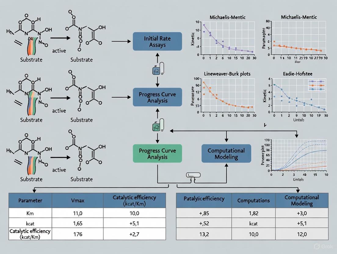
Estimating enzyme kinetic parameters, such as the turnover number ((k{cat})) and the Michaelis constant ((KM)), is fundamental to understanding catalytic efficiency and enzyme function in both basic research and drug development. For over a century, the Michaelis-Menten equation has served as the cornerstone for analyzing enzyme kinetics. The two primary experimental assays for parameter estimation are the initial velocity assay (initial rate analysis) and the reaction progress curve assay (progress curve analysis). The initial velocity method measures the rate of reaction immediately after mixing enzyme and substrate, relying on the linear portion of the progress curve. In contrast, the progress curve analysis fits the entire timecourse of substrate consumption or product formation to an integrated rate equation. This guide provides an objective comparison of these two traditional methods, detailing their protocols, data analysis, and appropriate applications to inform research and development workflows.
Core Principles and Methodological Comparison
Initial Velocity Assay
The initial velocity assay involves measuring the initial rates of the reaction ((v_0)) over a range of substrate concentrations. The underlying principle is that, under conditions of substrate saturation, the velocity of the catalyzed reaction is directly proportional to the enzyme concentration. This method requires that the initial rate is measured during the steady-state period, where the enzyme-substrate intermediate concentration remains approximately constant, and only a small fraction of the substrate has been consumed.
- Key Assumption: The approximation that the amount of free substrate is nearly equal to the initial substrate amount is valid because measurements are taken over a very short period with a large excess of substrate.
- Historical Context: Initial rate experiments are the simplest to perform and analyze and are relatively free from complications such as back-reaction and enzyme degradation, making them the most commonly used type of experiment in enzyme kinetics [25].
Progress Curve Assay
The progress curve assay determines kinetic parameters from expressions for species concentrations as a function of time. The concentration of substrate or product is recorded from the initial fast transient period until the reaction approaches equilibrium. This method uses the entire progress curve, fitting the data to the solution of a differential equation or an integrated rate equation.
- Key Assumption: The model used to fit the progress curve must accurately describe the enzyme's behavior throughout the reaction. Recent advances suggest that models derived with the total quasi-steady-state approximation (tQ) are accurate over a wider range of conditions, including when enzyme concentrations are not negligible compared to substrate concentrations, unlike the traditional standard QSSA (sQ) model [26].
- Modern Context: Although more technically challenging, the progress curve assay uses data more efficiently than the initial velocity assay [26].
Table 1: Core Methodological Comparison of Initial Velocity and Progress Curve Assays
| Feature | Initial Velocity Assay | Progress Curve Assay |
|---|---|---|
| Basic Principle | Measures initial reaction rates ((v_0)) at different substrate concentrations [27] [25] | Fits the complete timecourse of the reaction (progress curve) to a kinetic model [26] [28] |
| Primary Data Output | Initial velocity ((v_0)) vs. substrate concentration ([S]) plot [25] | Progress curve of product formation ([P]) or substrate consumption ([S]) over time (t) [26] |
| Data Analysis Method | Linear transforms (e.g., Lineweaver-Burk) or direct nonlinear fitting of the Michaelis-Menten equation to initial rates [26] | Nonlinear fitting of the complete progress curve to an integrated rate equation (e.g., Michaelis-Menten or tQ model) [26] [28] |
| Fundamental Requirement | Substrate must be in large excess over enzyme; only the initial, linear part of the reaction is used [27] [25] | The kinetic model must be valid for the entire course of the reaction, including non-linear phases [26] [28] |
Experimental Protocols and Data Analysis
Initial Velocity Assay Protocol
- Reaction Mixture Preparation: Prepare a series of reactions with a fixed, known concentration of enzyme and varying concentrations of substrate. The initial substrate concentration should range from values well below the anticipated (K_M) to values well above it to observe saturation.
- Initiation and Monitoring: Initiate the reaction by adding the enzyme. For continuous assays, immediately begin monitoring the formation of product or consumption of substrate over time using an appropriate method (e.g., spectrophotometry, fluorometry).
- Initial Rate Determination: Record the change in signal (e.g., absorbance, fluorescence) for a short period after the steady state is established but before a significant fraction (typically <5-10%) of the substrate has been consumed. The slope of the linear part of this progress curve is the initial velocity, (v_0) [27] [25].
- Replication: Repeat steps 1-3 for each substrate concentration in the series.
Progress Curve Assay Protocol
- Single Reaction Setup: Prepare a reaction mixture with a fixed concentration of enzyme and a single initial concentration of substrate.
- Continuous Monitoring: Initiate the reaction and continuously monitor the product formation or substrate consumption until the reaction approaches equilibrium or the signal stabilizes. This generates a full progress curve [28].
- Model Fitting: Fit the obtained progress curve data to an appropriate kinetic model. The traditional model is the integrated form of the Michaelis-Menten equation (sQ model). However, for greater accuracy, especially when enzyme concentration is not negligible, the model derived with the total quasi-steady-state approximation (tQ model) is recommended [26]. The tQ model is described by: ( \dot{P} = k{cat} ET \frac{(ET + KM + ST - P) - \sqrt{(ET + KM + ST - P)^2 - 4 ET (ST - P)}}{2} ) where ( \dot{P} ) is the production formation rate, (ET) is total enzyme concentration, (ST) is total initial substrate concentration, and (P) is the product concentration [26].
Comparative Data Analysis Workflow
The following diagram illustrates the logical flow of data analysis for both methods, highlighting key differences and decision points.
Performance and Application Analysis
Comparative Advantages and Limitations
The choice between initial velocity and progress curve assays involves trade-offs between experimental simplicity, data efficiency, and analytical rigor.
Table 2: Comparative Analysis of Assay Performance and Practical Considerations
| Aspect | Initial Velocity Assay | Progress Curve Assay |
|---|---|---|
| Data & Resource Efficiency | Requires many separate reaction runs to profile multiple [S]; can be substrate-intensive [26] | Can estimate parameters from a single progress curve; uses data more efficiently; less substrate required per parameter estimate [26] [28] |
| Parameter Identifiability | Requires [S] range from below to far above KM (often >10x KM) for reliable estimation, which can be difficult to achieve [26] [28] | Parameters can be identifiable with [S] around the KM level; optimal experiment design is simpler without prior KM knowledge [26] |
| Validity Conditions & Robustness | Validity of Michaelis-Menten equation requires enzyme concentration much lower than substrate + KM [26]. Simple and robust when conditions are strictly met. | The tQ model is accurate over wider conditions, including when enzyme concentration is not low [26]. More robust for in vivo-like conditions. |
| Handling of Non-Ideality | Only uses initial linear phase, avoiding complications like product inhibition or enzyme inactivation. | The full curve can be sensitive to non-idealities (e.g., inhibition, inactivation), which can be incorporated into more complex models for diagnosis [28]. |
| Technical & Computational Demand | Experimentally straightforward; data analysis is simple (linear or basic nonlinear regression) [25] | Requires high-quality continuous data; computational fitting is more complex, often requiring Bayesian inference or advanced algorithms [26] |
Supporting Experimental Data
A 2017 study systematically evaluated parameter estimation using Bayesian inference based on the standard QSSA (sQ) model (foundation of initial velocity analysis) and the total QSSA (tQ) model (suited for progress curve analysis). The study found that estimates obtained with the sQ model were "considerably biased when the enzyme concentration was not low," a restriction not required for the tQ model. Furthermore, the progress curve approach with the tQ model enabled accurate and precise estimation of kinetic parameters for diverse enzymes like chymotrypsin, fumarase, and urease from a minimal amount of timecourse data [26].
Another study highlighted that estimating enzyme activity through linear regression of the initial rate should only be applied when linearity is true, which is often not checked. In contrast, kinetic models for progress curve analysis can estimate maximum enzyme activity whether or not linearity is achieved, as they integrally account for the complete progress curve [28].
The Scientist's Toolkit: Essential Research Reagents and Materials
Successful execution of either kinetic assay requires careful control of experimental conditions and the use of specific reagents.
Table 3: Key Research Reagent Solutions for Enzyme Kinetics Assays
| Reagent/Material | Function in Assay | Key Considerations |
|---|---|---|
| Buffers (e.g., MES, Phosphate) | Maintain constant pH, crucial for enzyme activity and stability [29] [28] | Choice of buffer type and ionic strength is critical; each enzyme has an optimal pH [29]. |
| Cofactors (e.g., NADH, Thiamine Pyrophosphate) | Essential for the catalytic activity of many enzymes; often act as cosubstrates [28] | Must be added at saturating concentrations to avoid becoming rate-limiting. |
| Spectrophotometer / Fluorometer | Instrument for continuous monitoring of reaction progress via absorbance or fluorescence change [25] | Must have precise temperature control (≤±0.1°C), as a 1°C change can cause 4-8% activity variation [29]. |
| Discrete Analyzer / Automated System | Performs automated reagent additions and measurements in discrete, low-volume cuvettes [29] | Eliminates edge effects and offers superior temperature control, improving reproducibility for high-quality progress curves [29]. |
| Stopping Agent (for discontinuous assays) | Halts the reaction at precise times for product quantification (e.g., by HPLC) [29] | Used if continuous monitoring is not feasible; requires careful validation of quenching efficiency [29]. |
| Pure Enzyme / Crude Extract | The catalyst of interest. | Specific activity should be determined; crude extracts require controls for interfering activities [28] [25]. |
Both initial velocity and progress curve assays are vital tools for elucidating enzyme kinetics. The initial velocity assay remains the gold standard for its simplicity and robustness when ideal conditions (low enzyme, high substrate) can be met, making it excellent for routine characterization. The progress curve assay, particularly when employing more accurate kinetic models like the tQ model, offers a powerful, data-efficient alternative. It reduces experimental burden, is valid under a broader range of conditions (including high enzyme concentrations relevant to in vivo contexts), and can provide more precise parameter estimates from minimal data.
For researchers and drug development professionals, the selection criteria are clear: choose the initial velocity method for straightforward, traditional analysis under defined in vitro conditions. Opt for progress curve analysis when dealing with precious materials, when enzyme concentration is high, when seeking highly precise parameter estimates, or when aiming to detect and model more complex kinetic phenomena. The ongoing development of automated analysis systems and sophisticated computational packages for Bayesian inference is making progress curve analysis increasingly accessible and reliable, positioning it as a cornerstone of modern enzyme kinetics research.
The accurate estimation of enzyme kinetic parameters is a cornerstone of quantitative biology and drug development. For decades, the standard Quasi-Steady-State Approximation (sQSSA), leading to the classic Michaelis-Menten equation, has been the default model for analyzing enzyme-catalyzed reactions. However, its application is restricted to idealized conditions of low enzyme concentration, limiting its utility for studying modern experimental systems, including intracellular environments. This comparison guide evaluates the Total Quasi-Steady-State Approximation (tQSSA) as a superior alternative for parameter estimation. We provide a direct, data-driven comparison of their performance, experimental validation protocols, and practical applications, contextualizing their use within contemporary enzyme kinetics research.
Enzyme kinetic parameters—the Michaelis constant ((KM)), the catalytic rate constant ((k{cat})), and the dissociation constant ((Kd))—are fundamental for characterizing enzyme function, understanding metabolic pathways, and screening potential therapeutic inhibitors. The traditional method for estimating these parameters relies on the sQSSA, which is valid only under the condition that the total enzyme concentration is much lower than the total substrate concentration and the Michaelis constant ((ET \ll ST + KM)) [30] [31]. In vitro experiments often satisfy this condition, but it is frequently violated in vivo and in many modern experimental setups, such as those involving enzyme excess [32] [33].
When the sQSSA is applied outside its validity domain, it leads to systematic errors in parameter estimation, distorting the true catalytic efficiency and binding affinity of the enzyme. The tQSSA was developed to overcome this limitation. By redefining the reaction's slow variable to the total substrate concentration, it provides a mathematically rigorous and more accurate approximation across a vastly broader range of enzyme and substrate concentrations [30] [31] [33]. This guide objectively compares these two approaches, providing researchers with the data and methodologies needed to select the optimal tool for accurate kinetic characterization.
Theoretical and Practical Performance Comparison
The core difference between the sQSSA and tQSSA lies in their choice of the slow variable and the resulting form of the governing equations. The sQSSA assumes the free substrate concentration is the slow variable, while the tQSSA uses the total substrate concentration (( \bar{S} = S + C )), which is a conserved quantity [31]. This simple change in perspective resolves the mathematical stiffness that plagues the sQSSA under conditions of high enzyme concentration.
Validity Domains and Estimation Accuracy
The following table summarizes the key differences in the validity and performance of the two approximation methods.
Table 1: Comparative Analysis of sQSSA and tQSSA
| Feature | Standard QSSA (sQSSA) | Total QSSA (tQSSA) |
|---|---|---|
| Validity Condition | ( ET \ll ST + K_M ) [30] | Broadly valid for low and high enzyme concentrations (( ET \ll ST + KM ) and ( ST \ll ET + KM )) [30] [33] |
| Primary Limitation | Fails under high enzyme concentrations [31] | More complex mathematical formulation [31] |
| Accuracy in Deterministic Simulations | Poor outside its validity domain, can distort dynamics (e.g., dampen oscillations) [34] | Excellent across a wide parameter range; captures true system dynamics more reliably [34] [32] |
| Accuracy in Stochastic Simulations | Can be inaccurate even with timescale separation; accuracy depends on sensitivity of rate functions [34] | Generally more accurate than sQSSA, but not universally valid; can still distort dynamics in some stochastic systems [35] [36] |
| Parameter Estimation Fidelity | Tends to overestimate parameter values when (E_T) is significant [32] | Provides estimates much closer to real values, especially when (E_T) is not negligible [32] |
| Best-Suited For | Traditional in vitro assays with low enzyme concentrations. | In vivo modeling, high-throughput assays, and systems with any enzyme-to-substrate ratio. |
The superior accuracy of the tQSSA in deterministic contexts is well-established. For instance, in a genetic negative feedback model, the sQSSA reduced a limit cycle to damped oscillations, while the tQSSA correctly preserved the original system's oscillatory dynamics [34]. Furthermore, in "reverse engineering" tasks where models are fit to data to find unknown parameters, using the tQSSA yields estimates that are significantly closer to the true values, whereas the sQSSA "overestimates the parameter values greatly" [32].
A Note on Stochastic Simulations
A critical consideration for modern systems biology is the performance of these approximations in stochastic models, which are essential when molecular copy numbers are low. While the deterministic tQSSA is more robust than the sQSSA, recent research cautions against assuming this superiority automatically transfers to stochastic simulations.
The validity of the stochastic tQSSA depends not only on timescale separation but also on the sensitivity of the nonelementary reaction rate functions to changes in the slow species [34] [35]. The tQSSA results in less sensitive functions than the sQSSA, which generally makes it more accurate. However, applying the deterministic tQSSA directly to define propensity functions in stochastic simulations can sometimes distort dynamics, even when the deterministic approximation itself is valid [35] [36]. This highlights the need for caution and verification when using any deterministic QSSA for stochastic model reduction.
Experimental Protocols for Kinetic Parameter Estimation
This section outlines detailed methodologies for estimating kinetic parameters using both the sQSSA and tQSSA, enabling researchers to implement and compare these techniques directly.
Traditional Protocol: Initial Rate Analysis with sQSSA
The sQSSA protocol is the classic method found in most biochemistry textbooks.
- Experiment: Perform a series of reactions with a fixed, low concentration of enzyme ((ET)) and varying concentrations of substrate ((ST)). The condition (ET \ll ST) must be maintained for all data points used in the fit.
- Measurement: Measure the initial velocity ((v_0)) of product formation for each substrate concentration.
- Analysis: Fit the Michaelis-Menten equation, ( v0 = \frac{V{max} [S]}{KM + [S]} ), to the ((v0), ([S])) data, where ([S]) is the free substrate concentration (often approximated by (ST) when (ET) is low). (V{max}) and (KM) are the fitted parameters.
- Calculation: Calculate (k{cat}) from (V{max} = k{cat} ET).
This workflow is based on the established sQSSA theory described in the search results [30] [31].
Advanced Protocol: Full Time-Course Analysis with tQSSA
The tQSSA leverages modern computational power to fit parameters directly from the full progress curve, which is more robust and works under a wider range of conditions.
- Experiment: Conduct a single reaction (or preferably a few for validation) with known initial concentrations of enzyme ((ET)) and substrate ((ST)). The ratio can be arbitrary, including (ET \approx ST) or (ET > ST).
- Measurement: Continuously monitor the concentration of product (P(t)) or total substrate (\bar{S}(t)) over time to obtain a full progress curve.
- Model Definition: Use the tQSSA rate equation derived from the reversible Michaelis-Menten scheme: [ \frac{d\bar{S}}{dt} = -k2 C + k{-2} (ET - C)(ST - \bar{S}) ] where the complex concentration (C) is defined implicitly by the solution of the quadratic equation: [ C = \frac{(ET + KM + \sigma) - \sqrt{(ET + KM + \sigma)^2 - 4 ET \sigma}}{2} ] and (\sigma \equiv \bar{S} + (k{-2}/k1)(ST - \bar{S})) [31].
- Parameter Fitting: Use non-linear regression to fit the parameters (k1), (k{-1}), (k2), and (k{-2}) (and thus (KM) and (k{cat})) directly to the experimental progress curve (P(t)) or (\bar{S}(t)) by numerically integrating the tQSSA ordinary differential equation (ODE).
This total QSSA-based sequential method for estimating all kinetic parameters of the reversible Michaelis-Menten scheme has been demonstrated as a robust alternative to traditional methods [30] [31].
The Scientist's Toolkit: Essential Research Reagent Solutions
The following table details key reagents and computational tools required for implementing the tQSSA estimation protocol.
Table 2: Key Research Reagents and Tools for tQSSA Implementation
| Item Name | Function/Description |
|---|---|
| Purified Enzyme Preparation | High-purity enzyme at known concentration for setting up reactions with precise (E_T). |
| Stopped-Flow Spectrophotometer | Instrument for rapidly mixing enzyme and substrate and monitoring rapid, early reaction kinetics. |
| Quenched-Flow Instrument | Apparatus for halting a reaction at precise millisecond timescales for chemical analysis of intermediates. |
| Computational Software (e.g., R, Python, MATLAB) | Platform for numerically integrating the tQSSA ODE and performing non-linear regression analysis. |
| Fluorescent/Luminescent Substrate Analog | A substrate that generates a detectable signal upon conversion, enabling continuous progress curve monitoring. |
Decision Workflow and Comparative Analysis Diagrams
To aid in selecting the appropriate method, use the following decision workflow. The subsequent diagram illustrates the core conceptual difference between the two approximations.
Diagram 1: QSSA Selection Workflow
Diagram 2: Conceptual Framework of sQSSA vs. tQSSA
The Total Quasi-Steady-State Approximation represents a significant advancement in enzyme kinetics, effectively overcoming the limitations of the classic sQSSA. While the sQSSA remains a valid tool for simple, traditional assays, the tQSSA offers a more powerful and flexible framework for accurate parameter estimation across a wide spectrum of experimental conditions, including those relevant to drug development and systems biology. By adopting the tQSSA and the associated full time-course analysis protocol, researchers can achieve more reliable and accurate kinetic characterizations, leading to better predictive models and a deeper understanding of enzymatic mechanisms.
The accurate prediction of enzyme kinetic parameters—the turnover number (kcat), the Michaelis constant (Km), and the inhibition constant (Ki)—is a cornerstone of understanding and engineering biological systems. These parameters are pivotal for applications in metabolic engineering, drug discovery, and the development of biocatalysts. Traditionally, their determination has relied on costly, time-consuming experimental assays, creating a major bottleneck. The disparity between the millions of known enzyme sequences and the thousands with experimentally measured kinetics underscores this challenge [5]. Machine learning (ML), particularly deep learning, has emerged as a powerful tool to bridge this gap. By learning complex patterns from existing biochemical data, ML models can provide rapid, in silico estimates of kinetic parameters, thereby accelerating research and development. This guide objectively compares the performance and methodologies of several state-of-the-art ML frameworks, including the newly introduced CatPred, UniKP, CataPro, and others, providing researchers with the data needed to select the optimal tool for their work.
A diverse set of computational frameworks has been developed, each with distinct architectural philosophies and input requirements.
CatPred is a comprehensive deep learning framework designed to predict kcat, Km, and Ki. It explicitly addresses key challenges in the field, such as the evaluation of model performance on out-of-distribution enzyme sequences and the provision of reliable, query-specific uncertainty quantification for its predictions. It explores diverse feature representations, including pretrained protein language models (pLMs) and 3D structural features [5] [37].
UniKP is a unified framework that also predicts kcat, Km, and catalytic efficiency (kcat/Km). It leverages pretrained language models for both enzyme sequences (ProtT5) and substrate structures (SMILES transformer). Its machine learning module employs an ensemble model (Extra Trees) that was selected after a comprehensive comparison of 16 different ML models. A derivative framework, EF-UniKP, incorporates environmental factors like pH and temperature [38].
CataPro is another neural network-based framework that uses ProtT5 for enzyme sequence embedding and combines MolT5 embeddings with MACCS keys fingerprints for substrate representation. A key feature of CataPro is its rigorous evaluation on unbiased datasets, created by clustering enzyme sequences to ensure no test enzyme is highly similar to any training enzyme, thus providing a more realistic assessment of generalization ability [15].
ENKIE takes a different approach by employing Bayesian Multilevel Models (BMMs). Instead of using raw sequence or structure data, it leverages categorical predictors like Enzyme Commission (EC) numbers, substrate identifiers, and protein family annotations. This results in an inherently interpretable model that provides well-calibrated uncertainty estimates [39].
Specialized Architectures also exist for specific challenges. For instance, a three-module ML framework was developed to predict the temperature-dependent kcat/Km of β-glucosidase. This framework decomposes the problem into predicting the optimum temperature, the efficiency at that temperature, and the relative efficiency profile across temperatures [40].
The following diagram illustrates a generalized workflow common to many of these deep learning frameworks, from data input to final prediction.
Performance Comparison: A Quantitative Analysis
Benchmarking these tools reveals their respective strengths and weaknesses across different kinetic parameters and evaluation scenarios. The coefficient of determination (R²) and Pearson Correlation Coefficient (PCC) are common metrics, with higher values indicating better predictive performance.
Table 1: Prediction Performance forkcat
| Framework | Core Model Architecture | Test R² | Test PCC | Key Evaluation Context |
|---|---|---|---|---|
| CatPred [5] | Deep Learning (pLM/3D features) | Competitive | N/A | Out-of-distribution & with uncertainty |
| UniKP [38] | Extra Trees (with pLM features) | 0.68 | 0.85 | Random split (vs. DLKcat baseline) |
| CataPro [15] | Neural Network (pLM/fingerprints) | N/A | ~0.41 (for kcat/Km) | Unbiased, sequence-split validation |
| ENKIE [39] | Bayesian Multilevel Model | 0.36 | N/A | Extrapolation to new reactions |
Table 2: Prediction Performance forKm
| Framework | Core Model Architecture | Test R² | Test PCC | Key Evaluation Context |
|---|---|---|---|---|
| CatPred [5] | Deep Learning (pLM/3D features) | Competitive | N/A | Out-of-distribution & with uncertainty |
| UniKP [38] | Extra Trees (with pLM features) | Similar to baseline | N/A | Uses dataset from Kroll et al. |
| ENKIE [39] | Bayesian Multilevel Model | 0.46 | N/A | Extrapolation to new reactions |
A critical differentiator among frameworks is their approach to evaluation. While some models report high performance on random train-test splits, others use more rigorous "unbiased" or "out-of-distribution" splits where test enzymes share low sequence similarity with training enzymes. For example, CataPro employs a sequence-similarity clustering (40% identity cutoff) to create its test sets, ensuring a tougher and more realistic assessment of its generalization capability [15]. CatPred also highlights its robust performance on out-of-distribution samples, a scenario where pretrained protein language model features are particularly beneficial [5].
Furthermore, UniKP demonstrated a significant 20% improvement in R² over an earlier model, DLKcat, on a standard kcat prediction task [38]. Meanwhile, ENKIE achieves performance comparable to more complex deep learning models while using only categorical features, and it provides well-calibrated uncertainty estimates that increase when predictions are made for reactions or enzymes distant from the training data [39].
Experimental Protocols: How the Frameworks Are Built and Tested
The development of a robust predictive framework follows a multi-stage process, from data curation to final validation. The methodologies cited in the performance comparisons are built upon detailed experimental protocols.
Data Curation and Preprocessing
The foundation of any model is its data. Most frameworks source their initial data from public kinetic databases like BRENDA and SABIO-RK [5] [15] [39].
- Substrate Mapping: A critical step is the accurate mapping of substrate names to their chemical structures. This is typically done by converting common names to canonical SMILES strings using databases like PubChem, ChEBI, or KEGG [5].
- Sequence Retrieval: Enzyme sequences are obtained from UniProt using provided identifiers [15].
- Data Filtering: Entries with missing sequence or substrate information are filtered out. Some studies impose additional criteria to reduce measurement noise, though CatPred notes this can lead to information loss and bias [5].
Feature Representation
A key step is converting raw inputs into numerical features.
- Enzyme Representation: Most modern frameworks (CatPred, UniKP, CataPro) use embeddings from pretrained protein Language Models (pLMs) like ProtT5-XL-UniRef50. These models convert an amino acid sequence into a fixed-length vector that captures complex semantic and syntactic information [5] [15] [38].
- Substrate Representation: Common methods include:
Model Training and Evaluation
- Unbiased Evaluation: To prevent inflated performance metrics, CataPro and others use sequence-based splitting. Enzymes are clustered by sequence similarity (e.g., 40% identity), and clusters are assigned to training or test sets, ensuring no high-similarity sequences are shared between sets [15].
- Uncertainty Quantification: CatPred and ENKIE incorporate methods to estimate prediction uncertainty. CatPred uses probabilistic regression to distinguish between aleatoric (data noise) and epistemic (model uncertainty) variances, while ENKIE's Bayesian framework naturally provides posterior distributions [5] [39].
The following diagram illustrates the specialized three-module architecture designed for predicting enzyme activity across different temperatures, a complexity that single-module models struggle to capture.
The development and application of these ML frameworks rely on a suite of public databases, software tools, and computational resources.
| Resource Name | Type | Function in Research | Relevance to Frameworks |
|---|---|---|---|
| BRENDA [5] [15] [39] | Database | Primary source of experimentally measured enzyme kinetic parameters. | Used as a core training data source for all major frameworks. |
| SABIO-RK [5] [15] [39] | Database | Repository for biochemical reaction kinetics. | Another key data source for model training and validation. |
| UniProt [15] [39] | Database | Provides comprehensive protein sequence and functional information. | Used to retrieve amino acid sequences for enzymes in the datasets. |
| PubChem [5] [15] | Database | Repository of chemical molecules and their biological activities. | Used to map substrate names to canonical SMILES strings. |
| ProtT5 [15] [38] | Pre-trained Model | Protein language model that generates numerical embeddings from sequences. | Used by UniKP, CataPro, and CatPred for enzyme feature representation. |
| SMILES Transformer [38] | Pre-trained Model | Language model that generates embeddings from SMILES strings. | Used by UniKP for substrate feature representation. |
| MACCS Keys [15] | Molecular Fingerprint | A set of 166-bit structural keys for representing molecular features. | Used by CataPro as part of its substrate representation. |
| CD-HIT [15] | Software Tool | Tool for clustering biological sequences to reduce redundancy. | Used by CataPro to create unbiased train/test splits. |
The advent of deep learning frameworks like CatPred, UniKP, and CataPro marks a significant leap forward in the computational prediction of enzyme kinetics. While they share common goals, their comparative analysis reveals distinct strengths: CatPred's emphasis on uncertainty quantification and out-of-distribution robustness, UniKP's strong overall performance and flexibility with environmental factors, CataPro's rigorous generalization on unbiased splits, and ENKIE's interpretability and calibrated uncertainties with minimal input data.
For researchers, the choice of tool depends on the specific application. For high-confidence predictions on novel enzyme sequences, a framework with robust out-of-distribution testing and uncertainty estimates is crucial. For tasks involving environmental conditions, EF-UniKP is currently a leading option. The field continues to evolve rapidly, with future progress likely hinging on larger and more standardized datasets, improved integration of physical constraints, and methods that offer greater interpretability to guide experimental design. These tools are poised to become indispensable assets in the toolkit of researchers and drug developers, accelerating the cycle of discovery and engineering in biochemistry.
The accurate estimation of enzyme kinetic parameters is a cornerstone of enzymology, metabolic engineering, and drug discovery. Traditional experimental methods for determining parameters such as ( k{cat} ) (turnover number) and ( Km ) (Michaelis constant) are often cost and time-intensive, creating a significant bottleneck in enzyme characterization [5]. The rapid expansion of protein sequence and structural data has catalyzed the development of computational methods to bridge this gap. At the heart of these advances lies feature representation—the process of transforming raw protein data into meaningful numerical descriptors that machine learning (ML) models can interpret. Two dominant paradigms have emerged: protein Language Models (pLMs) that learn evolutionary patterns from vast sequence databases, and 3D structural approaches that leverage the spatial arrangement of atoms and residues. This guide provides a comparative analysis of these feature representation strategies, offering researchers a framework for selecting appropriate methodologies for enzyme kinetic parameter estimation.
Comparative Analysis of Feature Representation Methodologies
Protein Language Models (pLMs) for Sequence-Based Feature Extraction
Protein Language Models represent a transformative approach to feature extraction by learning contextual representations of amino acid sequences through self-supervised training on millions of protein sequences.
- Architecture and Training: pLMs such as ESM2, ESM3, and ProtT5 are trained on massive sequence databases (e.g., UniRef) to predict masked amino acids in sequences [41] [5]. This process forces the model to learn the underlying biochemical and evolutionary constraints that shape protein sequences. The resulting embeddings are dense numerical vectors that encode complex, contextual information about each residue and the overall protein fold.
- Application in Kinetic Prediction: In frameworks like CatPred, pLM-derived features serve as input for deep learning models predicting ( k{cat} ), ( Km ), and inhibition constant (( K_i )) [5]. A key advantage is their robustness on out-of-distribution samples—enzymes with low sequence similarity to those in the training data. This suggests pLMs learn generalizable patterns of enzyme function rather than memorizing training examples.
- Motion Prediction: The SeaMoon method demonstrates that pLM embeddings can predict continuous protein motions directly from sequence [41]. By inputting embeddings from structure-aware pLMs like ESM3 or ProstT5 into a convolutional neural network, SeaMoon predicts residue displacement vectors that capture functional conformational changes, a factor influencing enzyme kinetics.
3D Structural Descriptors for Spatial Feature Encoding
In contrast to sequence-based methods, 3D structural descriptors explicitly represent the spatial atomic coordinates of a protein, aiming to capture the physical and chemical environment of the active site.
- Graph Neural Networks (GNNs): Methods like TopEC represent protein structures as 3D graphs where nodes are atoms or residues, and edges represent spatial relationships [42]. Message-passing frameworks such as SchNet and DimeNet++ incorporate inter-atomic distances and angles to create a detailed model of the local chemical environment. TopEC uses a localized descriptor focused on the enzyme's binding site, which reduces computational complexity and focuses learning on the functionally relevant region.
- Template-Based Methods: Older approaches, such as the Evolutionary Trace Annotation (ETA) pipeline, constructed 3D templates from evolutionarily critical residues to identify functional similarities across diverse protein structures [43]. While conceptually different from deep learning, it highlights the enduring principle that local spatial geometry is a strong indicator of function.
- Challenges: A significant limitation of 3D structural methods is their dependence on high-quality protein structures, which may not be available for all proteins of interest. Furthermore, atomistic graphs are computationally demanding, often requiring significant GPU memory [42].
Integrated Approaches Combining pLMs and Structural Features
The most recent and powerful frameworks combine pLM and 3D structural features to leverage the strengths of both paradigms.
- The CatPred Framework: CatPred explores diverse learning architectures and feature representations, including both pretrained pLMs and 3D structural features [5]. This hybrid approach allows the model to benefit from the evolutionary information in pLM embeddings and the physico-chemical context from 3D structures. The framework provides accurate predictions with query-specific uncertainty estimates, which is critical for applications in protein engineering and metabolic modeling.
- Performance in Kinetic Prediction: CatPred has been benchmarked on extensive datasets (~23,000 ( k{cat} ), ~41,000 ( Km ), and ~12,000 ( K_i ) data points) and demonstrates competitive performance [5]. Its probabilistic regression approach quantifies both aleatoric (data noise) and epistemic (model uncertainty) variances, offering guardrails on prediction reliability.
Table 1: Comparison of Feature Representation Methodologies for Enzyme Kinetic Prediction
| Method | Core Technology | Features Represented | Key Advantages | Primary Applications |
|---|---|---|---|---|
| pLMs (e.g., ESM2, ProtT5) | Transformer-based Neural Networks | Evolutionary patterns, sequence context, putative structure | Generalizability, works from sequence alone, fast inference | ( k{cat} )/( Km ) prediction (CatPred, UniKP), motion prediction (SeaMoon) |
| 3D Structural GNNs (e.g., TopEC) | Graph Neural Networks (SchNet, DimeNet++) | Inter-atomic distances, angles, local chemical environment | Explicit modeling of physical interactions and active site geometry | Enzyme Commission (EC) number prediction, functional annotation |
| Hybrid Models (e.g., CatPred) | Integrated pLM & Structural Features | Combined evolutionary and physico-chemical constraints | High accuracy, reliable uncertainty quantification, robust on diverse inputs | Comprehensive enzyme kinetic parameter estimation (( k{cat} ), ( Km ), ( K_i )) |
Experimental Protocols and Performance Benchmarking
Key Experimental Workflows
Understanding the experimental protocols is essential for evaluating the supporting data for each feature representation method.
- Workflow for 3D Graph-Based Prediction (TopEC): The TopEC protocol begins by generating a protein structure, either experimentally or via prediction tools like AlphaFold2 [42]. The binding site is identified using methods like P2Rank. A graph is constructed where nodes are atoms/residues within this localized region. The 3D GNN (SchNet for distances, DimeNet++ for distances and angles) then performs message-passing to learn a function-relevant representation. Finally, a classifier predicts the EC number. Benchmarking on a fold-split dataset (to remove bias from similar protein folds) showed TopEC achieved an F-score of 0.72 for EC classification, outperforming regular 2D GNNs [42].
- Workflow for pLM-Based Kinetic Prediction (CatPred): For a given enzyme-substrate pair, the enzyme sequence is passed through a pretrained pLM (e.g., ProtT5) to generate a feature embedding [5]. The substrate is typically represented using a molecular fingerprint or graph. These features are then fed into a deep learning regression model (e.g., CNN or ensemble) to predict the kinetic parameter. Crucially, CatPred uses probabilistic regression to output a predictive distribution, providing a mean prediction and an estimate of uncertainty. Evaluation shows that lower predicted variances correlate with higher prediction accuracy [5].
The following diagram illustrates the logical workflow for selecting a feature representation methodology, integrating both pLM and 3D structural approaches.
Quantitative Performance Comparison
Benchmarking studies provide critical data for comparing the performance of different feature representation approaches.
Table 2: Summary of Quantitative Performance Metrics from Key Studies
| Method / Framework | Feature Representation | Key Performance Metric | Reported Result | Experimental Context |
|---|---|---|---|---|
| TopEC [42] | 3D Graph Neural Network (localized binding site) | F-score (EC Classification) | 0.72 | Fold-split dataset (experimental & predicted structures) |
| CatPred [5] | pLM embeddings + 3D structural features | Accuracy / Uncertainty Quantification | Competitive performance; Lower predicted variance correlates with higher accuracy | Benchmark on ~23k ( k{cat} ), ~41k ( Km ), ~12k ( K_i ) data points |
| SeaMoon-ProstT5 [41] | pLM embeddings (ProstT5) | Normalized Sum-of-Squares Error (NSSE) | Success rate of 40% (NSSE < 0.6) | Prediction of protein motions from sequence on a test set of 1,121 proteins |
| ETA Pipeline [43] | Evolutionary Trace 3D templates | Annotation Accuracy | 87% accuracy (when a single function had a plurality of matches) | Benchmark on 98 enzymes from the Protein Structure Initiative |
This section details key databases, software tools, and computational resources that form the foundation for research in this field.
Table 3: Key Research Reagent Solutions for Feature Representation and Kinetic Modeling
| Item Name | Type | Function / Application | Relevant Citation |
|---|---|---|---|
| AlphaFold2 & ESMFold | Structure Prediction Tool | Generates 3D protein structures from amino acid sequences for use in structural feature extraction. | [44] [45] |
| BRENDA & SABIO-RK | Kinetic Database | Primary sources of curated experimental enzyme kinetic parameters (( k{cat} ), ( Km} ), ( K_i )) for model training and validation. | [5] |
| CatPred Framework | Software Framework | An integrated deep learning framework for predicting ( k{cat} ), ( Km ), and ( K_i ) using pLM and 3D features. | [5] |
| TopEC Software | Software Package | A 3D graph neural network for predicting Enzyme Commission (EC) classes from protein structures. | [42] |
| ESM2/ESM3 & ProtT5 | Protein Language Model | Generates state-of-the-art numerical embeddings from protein sequences for use in machine learning models. | [41] [5] |
| Protein Data Bank (PDB) | Structure Database | Repository of experimentally determined 3D structures of proteins, used for training and testing structural models. | [42] [43] |
| UniProt | Sequence Database | Comprehensive resource for protein sequence and functional information, used for training pLMs. | [5] |
The choice between protein Language Models and 3D structural data for feature representation is not a binary one. pLMs offer unparalleled speed and generalizability from sequence alone, making them ideal for high-throughput screening on vast genomic datasets. In contrast, 3D structural approaches provide a deeper, physico-chemical understanding of enzyme mechanism, which is valuable for detailed functional annotation and engineering. The most robust frameworks, such as CatPred, are now moving towards a hybrid paradigm that integrates the strengths of both worlds. For researchers focused on enzyme kinetic parameter estimation, this integration—complemented by reliable uncertainty quantification—represents the current state of the art, enabling more confident applications in drug development and metabolic engineering.
Accurate estimation of enzyme kinetic parameters is fundamental to understanding cellular systems, designing industrial biocatalysts, and advancing drug development. For over a century, the Michaelis-Menten equation has served as the cornerstone model for characterizing enzyme kinetics, describing reaction velocity (V) as a function of substrate concentration ([S]) via two fundamental parameters: the maximum reaction rate (Vmax) and the Michaelis constant (Km) [4]. Despite its widespread adoption, researchers face significant challenges in obtaining reliable parameter estimates, particularly when dealing with complex enzymatic systems that deviate from ideal Michaelis-Menten assumptions [46] [47].
This guide provides a comprehensive comparison of contemporary parameter estimation methodologies, from traditional linearization approaches to cutting-edge computational frameworks. We objectively evaluate the performance of various methods using published experimental data and simulation studies, with particular emphasis on the renz R package as a representative modern solution. By synthesizing recent advances in biochemical methodology, statistical analysis, and machine learning, we aim to equip researchers with practical workflows for robust kinetic parameter estimation across diverse experimental scenarios.
Fundamental Concepts and Historical Context
The Michaelis-Menten Framework
The canonical Michaelis-Menten model describes enzyme-catalyzed reactions through the equation:
[v = \frac{V{\text{max}} \cdot [S]}{Km + [S]}]
where (v) represents the initial reaction velocity, (V{\text{max}}) is the maximum reaction rate, ([S]) is the substrate concentration, and (Km) is the Michaelis constant equal to the substrate concentration at half (V{\text{max}}) [4]. The (Km) provides a measure of enzyme-substrate binding affinity, with lower values indicating stronger binding, while (k{cat}) (catalytic constant) relates to (V{\text{max}}) through the enzyme concentration ((V{\text{max}} = k{cat} \cdot E_T)) [47].
Limitations of Traditional Approaches
Historically, researchers employed linear transformations of the Michaelis-Menten equation to estimate kinetic parameters. The Lineweaver-Burk (double-reciprocal) plot and Eadie-Hofstee plot were particularly popular due to their simplicity and the familiarity of linear regression [4] [46]. However, these linearization methods present substantial statistical limitations, as they distort experimental error distribution and violate key assumptions of linear regression [4] [46] [48]. Studies have demonstrated that these approaches can yield widely varying parameter estimates, with some cases even producing nonsensical negative values for kinetic parameters [46].
Methodological Comparison: Estimation Approaches
Classification of Estimation Methods
Contemporary methods for estimating enzyme kinetic parameters can be categorized according to two key criteria: (1) whether they utilize single progress curves or initial velocity data, and (2) whether they employ data transformation or direct nonlinear regression [48]. Progress curve methods analyze the complete timecourse of substrate depletion or product formation, while initial velocity methods use rates calculated from the linear portion of progress curves at different substrate concentrations [48]. Methods that avoid data transformation preserve error distribution characteristics and typically provide more reliable parameter estimates [48].
Table 1: Classification of Enzyme Kinetic Parameter Estimation Methods
| Method Category | Data Requirement | Key Features | Limitations |
|---|---|---|---|
| Linear Transformation (e.g., Lineweaver-Burk, Eadie-Hofstee) | Initial velocities at varying [S] | Simple implementation; visual linear relationship | Error distortion; unreliable parameter estimates [4] [46] |
| Nonlinear Regression (Vi-[S] data) | Initial velocities at varying [S] | Direct fitting to Michaelis-Menten equation; better error handling | Requires multiple progress curves; potential parameter identifiability issues [4] [47] |
| Progress Curve Analysis ([S]-time data) | Single substrate timecourse | Efficient data usage; minimal experimental work | Complex integrated equations; requires numerical solution [4] [48] |
| Total QSSA-Based Methods | Single substrate timecourse | Accurate under wider enzyme:substrate ratios; suitable for in vivo conditions | Computationally intensive; less familiar to researchers [47] |
Performance Comparison of Estimation Methods
A comprehensive simulation study comparing five estimation methods revealed significant differences in accuracy and precision [4]. Researchers generated 1,000 replicates of simulated substrate concentration-time data incorporating additive or combined error models, then estimated Vmax and Km using different approaches.
Table 2: Performance Comparison of Estimation Methods Based on Simulation Studies [4]
| Estimation Method | Description | Relative Accuracy | Relative Precision | Performance with Combined Error |
|---|---|---|---|---|
| Lineweaver-Burk (LB) | Linear regression of 1/V vs 1/[S] | Low | Low | Poor |
| Eadie-Hofstee (EH) | Linear regression of V vs V/[S] | Low | Low | Poor |
| Nonlinear Regression (NL) | Direct nonlinear fit of V-[S] data | Moderate | Moderate | Moderate |
| Nonlinear Differential (ND) | Nonlinear fit of averaged rate data | Moderate | Moderate | Moderate |
| Nonlinear Mixed Effects (NM) | Nonlinear regression of [S]-time data | High | High | Superior |
The study demonstrated that nonlinear methods using specialized computational tools (e.g., NONMEM) provided the most accurate and precise parameter estimates, with particular superiority in handling complex error structures [4]. Traditional linearization methods consistently underperformed, especially with combined error models commonly encountered in experimental practice.
Diagram 1: Performance hierarchy of enzyme kinetic parameter estimation methods. Traditional linearization methods (red) show lowest accuracy, while modern nonlinear approaches (blue, green) provide progressively better performance.
The Renz Package: A Modern Solution
The renz package represents a contemporary approach designed to bridge the gap between highly specialized enzymatic modeling software and general-purpose graphing programs [48]. Implemented as a cross-platform, open-source R package, renz provides utilities for accurate and efficient estimation of enzyme kinetic parameters while maintaining accessibility for non-specialists [48]. The package compiles and runs on various UNIX platforms, Windows, and MacOS as a stand-alone program, requiring R (≥4.0.0) as a prerequisite [48].
Comparative Analysis Against Alternatives
Table 3: Software Solutions for Enzyme Kinetic Parameter Estimation
| Software | License | Platform Support | Stand-alone | Key Features |
|---|---|---|---|---|
| renz | Free open source | Cross-platform | Yes | Comprehensive Michaelis-Menten analysis; progress curve and initial rate methods [48] |
| ICEKAT | Free open source | Cross-platform | No | Browser-based; semi-automated initial rate calculations [48] |
| DynaFit | Free open source | Limited | Yes | Complex enzymatic mechanisms; global fitting [48] |
| KinTek | Commercial | Limited | Yes | Comprehensive kinetic modeling; parameter space exploration [48] |
| ENZO | Free open source | Cross-platform | No | Web-based tool; enzymatic data analysis [48] |
| NONMEM | Commercial | Limited | Yes | Nonlinear mixed effects modeling; population kinetics [4] |
Unlike specialized packages requiring complex model specification, renz focuses specifically on Michaelis-Menten kinetics while avoiding the limitations of general-purpose graphing software like GraphPad Prism or Microsoft Excel [48]. The package includes five detailed vignettes that guide users through method selection, theoretical foundations, and practical application with real experimental data [48].
Advanced Methodologies and Emerging Approaches
Bayesian Inference and Total QSSA Models
Recent advances have introduced Bayesian approaches based on the total quasi-steady-state approximation (tQSSA) to overcome limitations of traditional Michaelis-Menten analysis [47]. Unlike the standard QSSA (sQ) model, which requires enzyme concentration to be much lower than substrate concentration, the tQ model remains accurate across diverse enzyme:substrate ratios, making it particularly suitable for in vivo conditions where enzyme concentrations are typically higher [47].
Comparative studies demonstrate that estimates obtained with the tQ model exhibit little bias regardless of enzyme and substrate concentrations, while sQ model estimates show considerable bias when enzyme concentration is not low [47]. This approach enables experimental data from various conditions to be pooled without restrictions, improving estimation accuracy and precision [47].
Machine Learning and Deep Learning Frameworks
The emergence of large-scale kinetic datasets has enabled the development of machine learning approaches for predicting enzyme kinetic parameters. CatPred, a comprehensive deep learning framework, predicts in vitro enzyme kinetic parameters including turnover numbers (kcat), Michaelis constants (Km), and inhibition constants (Ki) [5]. This framework addresses key challenges such as performance evaluation on enzyme sequences dissimilar to training data and model uncertainty quantification [5].
CatPred utilizes diverse learning architectures and feature representations, including pretrained protein language models and three-dimensional structural features, to enable robust predictions [5]. The framework provides accurate predictions with query-specific uncertainty estimates, with lower predicted variances correlating with higher accuracy [5]. Similarly, EnzyExtract employs large language models to automatically extract, verify, and structure enzyme kinetics data from scientific literature, having processed 137,892 full-text publications to collect over 218,095 enzyme-substrate-kinetics entries [24].
Experimental Design Considerations
Optimal experimental design significantly improves parameter estimation precision. For progress curve assays, the initial substrate concentration is recommended to be at a similar level to Km, while initial velocity assays require substrate concentrations ranging from below to well above Km to ensure identifiability [47]. Research indicates that fed-batch processes can provide better estimation precision compared to batch processes, with optimal sampling strategies dramatically improving parameter confidence [49].
For initial velocity assays, the highest and lowest practically attainable substrate concentrations at equal frequency are generally favorable when relative measurement error is constant [49]. Computational approaches can determine optimal measurement points by maximizing the determinant of the Fisher information matrix, though these typically require rough parameter estimates beforehand [49].
Practical Applications and Case Studies
Experimental Protocol: β-Galactosidase Kinetics
A representative experimental analysis using β-galactosidase as an enzyme model illustrates the importance of proper methodological selection [46] [48]. When students analyzed kinetic data using conventional linear regression of double-reciprocal plots, the resulting Km and Vmax values varied widely, with some cases producing negative values [46]. However, when properly analyzed with weighted regression accounting for error propagation, the data yielded consistent parameter estimates (Km = 2.8 ± 0.3 mM; Vmax = 179 ± 27 mM/min) with reduced intergroup standard deviation [46].
Cross-Enzyme Validation Studies
Comprehensive validation across enzymes with disparate catalytic efficiencies demonstrates the robustness of modern estimation approaches. Studies examining chymotrypsin, fumarase, and urease have confirmed that Bayesian inference with tQ models enables accurate and precise parameter estimation from minimal timecourse data [47]. This approach facilitates the development of publicly accessible computational packages that perform efficient Bayesian inference for enzyme kinetics [47].
Diagram 2: Comprehensive workflow for enzyme kinetic parameter estimation, showing methodological choices and application areas.
Essential Research Reagents and Computational Tools
Table 4: Research Reagent Solutions for Enzyme Kinetic Studies
| Reagent/Resource | Function/Purpose | Example Applications |
|---|---|---|
| β-Galactosidase | Model enzyme for method validation | Educational labs; protocol optimization [46] [48] |
| o-Nitrophenyl-β-d-galactopyranoside (ONPG) | Chromogenic substrate for β-galactosidase | Kinetic assays with spectrophotometric detection [48] |
| renz R Package | Statistical analysis of kinetic data | Michaelis-Menten parameter estimation [48] |
| CatPred Framework | Deep learning prediction of kinetic parameters | kcat, Km, and Ki prediction from sequence [5] |
| EnzyExtract Database | LLM-curated kinetic parameters from literature | Data mining; model training [24] |
| NONMEM | Nonlinear mixed effects modeling | Population kinetics; complex error structures [4] |
The landscape of enzyme kinetic parameter estimation has evolved significantly from traditional linearization methods to sophisticated computational approaches. Our comparison demonstrates that nonlinear regression methods, particularly those analyzing progress curves directly, provide superior accuracy and precision compared to traditional linear transformations. The renz package represents an accessible yet powerful solution for researchers requiring reliable Michaelis-Menten parameter estimation, filling a crucial gap between oversimplified graphing software and excessively complex specialized packages.
Emerging methodologies including Bayesian inference with tQ models, deep learning frameworks like CatPred, and large-scale data extraction tools such as EnzyExtract are expanding the boundaries of what's possible in enzyme kinetics. These approaches enable robust parameter estimation across diverse experimental conditions, facilitate prediction from sequence information, and unlock the vast "dark matter" of enzymatic data scattered throughout scientific literature. As the field continues to advance, integration of these complementary approaches promises to accelerate research in drug development, metabolic engineering, and fundamental biochemical understanding.
Solving Common Challenges: Parameter Identifiability, Reliability, and Experimental Design
Addressing Parameter Unidentifiability in Complex Reactions
Enzyme kinetic parameter estimation is a fundamental process in biochemical research and drug development, enabling scientists to quantify how enzymes interact with substrates and inhibitors. The accurate determination of parameters such as kcat (catalytic constant) and KM (Michaelis-Menten constant) is essential for predicting enzyme behavior in various biological contexts. However, complex reaction mechanisms, particularly those involving multiple substrates or competing pathways, often present significant challenges through parameter unidentifiability. This phenomenon occurs when multiple combinations of parameter values can equally explain experimental data, making it impossible to determine unique, reliable values for the parameters of interest [50] [47].
The issue of identifiability is especially pronounced in enzymes like CD39/NTPDase1, which catalyze sequential reactions where the product of one reaction serves as the substrate for another. In such cases, traditional estimation methods often fail because parameters for individual steps cannot be distinguished from overall reaction progress data [50]. This review comprehensively compares contemporary methodologies for addressing parameter unidentifiability, providing experimental protocols, and evaluating performance across different enzymatic systems relevant to pharmaceutical research and development.
Fundamental Concepts and Challenges
Michaelis-Menten Framework and Its Limitations
The Michaelis-Menten equation has served as the cornerstone of enzyme kinetics for over a century. This model describes enzyme-catalyzed reaction rates through the equation v = Vmax[S] / (KM + [S]), where Vmax represents the maximum reaction rate, KM is the Michaelis constant, and [S] is the substrate concentration [8]. For single-substrate reactions under ideal conditions, this framework provides reliable parameter estimates. However, its application becomes problematic for complex enzymatic mechanisms involving multiple substrates or competing pathways [50].
The standard quasi-steady-state approximation (sQSSA) underlying traditional Michaelis-Menten kinetics requires that enzyme concentration be significantly lower than the sum of substrate concentration and KM (ET ≪ KM + ST) [47]. This condition frequently cannot be met in physiological environments where enzyme concentrations may approach or exceed substrate levels, leading to systematic errors in parameter estimation. Furthermore, graphical linearization methods such as Lineweaver-Burk plots have been shown to distort error structures and produce inaccurate parameter estimates, exacerbating identifiability issues [50].
Identifiability Challenges in Complex Reaction Systems
Complex enzymatic reactions present unique identifiability challenges that straightforward Michaelis-Menten analysis cannot address. The CD39/NTPDase1 enzyme exemplifies this problem, as it hydrolyzes ATP to ADP and subsequently ADP to AMP within a single catalytic pathway [50]. This substrate competition creates a situation where ADP serves simultaneously as a product and substrate, complicating the determination of individual kinetic parameters for each hydrolytic step.
Parameter unidentifiability in such systems arises from structural limitations in the mathematical models themselves. When parameters exhibit strong correlations or when the model structure allows multiple parameter combinations to produce identical experimental outputs, unique identification becomes impossible without additional constraints or experimental designs [50] [47]. This fundamental limitation necessitates advanced methodological approaches that can disentangle interdependent parameters through specialized experimental designs or computational methods.
Methodological Comparison for Identifiability Resolution
Traditional Linearization Methods
Traditional approaches to enzyme kinetic parameter estimation have relied heavily on linear transformation methods, including Lineweaver-Burk, Eadie-Hofstee, and Hanes-Woolf plots. These methods linearize the Michaelis-Menten equation to enable parameter estimation through linear regression [8]. While computationally straightforward, these approaches introduce significant statistical biases by distorting the error structure of the experimental data. The transformation process unevenly weights data points, potentially emphasizing less reliable measurements and compromising parameter accuracy [50].
The limitations of linearization methods become particularly pronounced in complex reaction systems. For CD39 kinetics, model simulations using parameter values obtained through linearization methods failed to align with experimental time-series data, demonstrating their inadequacy for resolving parameter identifiability in multi-step reactions [50]. This systematic misalignment highlights the fundamental insufficiency of these traditional approaches for complex enzymatic systems relevant to drug discovery.
Modern Computational Approaches
Nonlinear Least Squares Estimation
Nonlinear least squares (NLS) estimation represents a significant advancement over linearization methods by directly fitting the untransformed Michaelis-Menten equation to experimental data. This approach preserves the inherent error structure and provides more reliable parameter estimates under appropriate conditions [50]. However, NLS estimation still faces challenges with parameter correlations in complex reaction systems, where strong dependencies between KM and Vmax values can persist even with improved fitting techniques.
For the CD39 system, direct application of NLS estimation to the full reaction progress curves still resulted in unidentifiable parameters due to persistent interactions between the ATPase and ADPase kinetic parameters [50]. The residual sum of squares surface displayed a elongated valley where different parameter combinations yielded similarly good fits, indicating that NLS alone is insufficient for resolving identifiability issues in complex enzymatic pathways without additional experimental constraints.
Bayesian Inference Framework
Bayesian methods provide a powerful alternative for addressing parameter unidentifiability by incorporating prior knowledge and quantifying uncertainty in parameter estimates. This approach is particularly valuable when parameters are poorly identified from data alone, as it allows researchers to formally incorporate constraints based on mechanistic understanding or previous experiments [47].
When applied with the total quasi-steady-state approximation (tQ) model, Bayesian inference enables accurate parameter estimation across a wider range of enzyme and substrate concentrations compared to traditional methods [47]. The Bayesian framework naturally handles parameter correlations by exploring the joint posterior distribution of all parameters, providing a complete picture of identifiability issues rather than point estimates that may be misleading. This approach also facilitates optimal experimental design by identifying measurement conditions that maximize parameter identifiability.
Total Quasi-Steady-State Approximation (tQSSA)
The total quasi-steady-state approximation offers a fundamental improvement in enzyme kinetics modeling by expanding the range of conditions under which approximate solutions remain accurate. Unlike the standard QSSA, which requires ET ≪ KM + ST, the tQSSA remains valid under a broader set of conditions including high enzyme concentrations [47].
The tQ model describes product accumulation using the equation: dP/dt = kcat(ET + KM + ST - P - √[(ET + KM + ST - P)² - 4ET(ST - P)])/2
This more complex formulation provides superior accuracy across diverse enzyme-to-substrate ratios, making it particularly valuable for estimating kinetic parameters under physiologically relevant conditions where enzyme concentrations may be significant [47]. By maintaining accuracy across wider experimental conditions, the tQSSA reduces structural identifiability issues inherent in the traditional Michaelis-Menten framework.
Comparative Performance Analysis
Table 1: Comparison of Enzyme Kinetic Parameter Estimation Methods
| Method | Theoretical Basis | Identifiability Performance | Experimental Requirements | Computational Complexity |
|---|---|---|---|---|
| Linearization Methods | Transformed Michaelis-Menten equation | Poor for complex systems; biased parameter estimates | Multiple substrate concentrations; initial rate measurements | Low; linear regression |
| Nonlinear Least Squares | Direct fit to Michaelis-Menten equation | Improved but still unidentifiable for correlated parameters | Full time-course data | Moderate; iterative optimization |
| Bayesian Inference with sQ model | Standard QSSA with Bayesian estimation | Limited by sQSSA validity conditions | Data under low enzyme conditions | High; Markov Chain Monte Carlo sampling |
| Bayesian Inference with tQ model | Total QSSA with Bayesian estimation | Excellent across diverse conditions; handles parameter correlations | Flexible experimental designs | High; advanced computational methods |
The performance comparison reveals a clear progression in methodological sophistication, with Bayesian inference coupled with the tQ model providing the most robust solution to parameter unidentifiability. This approach enables reliable parameter estimation even when enzyme concentrations approach or exceed substrate levels, a common scenario in physiological systems and pharmaceutical testing [47].
For the CD39 system, the tQ model enabled accurate and precise estimation of kinetic parameters from a minimal amount of time-course data, successfully addressing the identifiability challenges that plagued traditional methods [50]. This combination of experimental design and computational methodology represents the current state-of-the-art for parameter estimation in complex enzymatic systems.
Experimental Protocols for Identifiability Resolution
Isolated Reaction Analysis Protocol
For enzymes with multiple catalytic steps or competing substrates, isolating individual reactions provides the most direct approach to resolving parameter identifiability. This method was successfully applied to CD39 kinetics by separately analyzing ATPase and ADPase activities [50].
Procedure:
- ATPase Reaction Isolation: Prepare reaction mixtures containing 500 μM ATP, recombinant enzyme, and reaction buffer. Omit ADP from initial reactions to prevent competitive inhibition.
- ADPase Reaction Isolation: Prepare separate reaction mixtures containing 500 μM ADP as the initial substrate without ATP present.
- Time-Course Sampling: Collect samples at regular intervals (e.g., 0, 5, 10, 15, 30, 45, 60 minutes) from both reaction sets.
- Analytical Measurement: Quantify substrate depletion and product formation using appropriate methods (HPLC, spectrophotometric assays, or radiometric detection).
- Independent Parameter Estimation: Fit the Michaelis-Menten model separately to the ATPase and ADPase time-course data using nonlinear regression.
- Global Model Validation: Combine the independently estimated parameters into the full kinetic model and validate against experimental data where both substrates are present.
This approach decouples interdependent parameters by obtaining initial estimates for each catalytic step in isolation, effectively breaking the correlation between parameters that causes unidentifiability in the full system [50].
Optimal Experimental Design for Parameter Identification
Strategic experimental design significantly enhances parameter identifiability by collecting data that provides maximal information about target parameters. The Bayesian framework facilitates this through pre-experimental analysis of potential data collection strategies [47].
Procedure:
- Preliminary Range-Finding Experiments: Conduct initial experiments across broad concentration ranges to identify approximate parameter values.
- Fisher Information Matrix Analysis: Calculate the Fisher information matrix for proposed experimental conditions to quantify expected parameter uncertainties.
- Optimal Design Selection: Choose substrate and enzyme concentrations that maximize the determinant of the Fisher information matrix, ensuring maximal parameter identifiability.
- Multi-Condition Data Collection: Collect progress curve data from optimally selected conditions, specifically including both low and high enzyme-to-substrate ratios.
- Pooled Data Analysis: Simultaneously fit all data sets using the tQ model to obtain final parameter estimates with minimized uncertainty.
This methodology enables efficient experimental design without requiring precise prior knowledge of kinetic parameters, overcoming the circular challenge of needing to know parameters to design experiments to estimate those same parameters [47].
Progress Curve Analysis with tQ Model
Comprehensive progress curve analysis using the tQ model provides robust parameter estimation across diverse experimental conditions, effectively addressing identifiability issues present in traditional approaches [47].
Procedure:
- Reaction Setup: Prepare enzyme-substrate mixtures across strategically chosen concentration ratios, specifically including conditions where enzyme concentration approaches or exceeds KM.
- Continuous Monitoring: Measure product formation or substrate depletion continuously or with high temporal resolution throughout reaction progress.
- Numerical Integration: Implement the tQ model differential equation using computational methods (MATLAB, Python, or specialized software).
- Parameter Estimation: Fit the model to progress curve data using maximum likelihood or Bayesian estimation methods.
- Identifiability Assessment: Compute profile likelihoods or Bayesian credible intervals to quantify parameter uncertainties and identify potential correlations.
- Model Validation: Compare model predictions with experimental data not used in parameter estimation to verify predictive capability.
This protocol leverages the broader validity of the tQ model compared to traditional Michaelis-Menten kinetics, enabling accurate parameter estimation from progress curve data even when enzyme concentrations are substantial [47].
Visualization of Methodological Relationships
Figure 1: Methodological evolution for addressing parameter unidentifiability, showing the progression from traditional approaches (yellow) to modern computational methods (green) and advanced theoretical frameworks (blue). Solid arrows indicate successful paths to identifiability resolution, while dashed lines represent approaches with limited effectiveness for complex systems.
Essential Research Reagent Solutions
Table 2: Key Research Reagents and Materials for Enzyme Kinetic Studies
| Reagent/Material | Function in Kinetic Studies | Application Examples | Considerations for Identifiability |
|---|---|---|---|
| Recombinant Enzymes | Catalytic component for reaction studies | CD39/NTPDase1, chymotrypsin, fumarase, urease | Purity and concentration critical for accurate parameter estimation |
| Nucleotide Substrates | Reactants for enzymatic conversion | ATP, ADP, AMP for nucleotidases | High purity to prevent competitive inhibition from contaminants |
| Spectrophotometric Assays | Continuous monitoring of reaction progress | NADH-linked assays, chromogenic substrates | Enables dense data collection for progress curve analysis |
| HPLC Systems | Discontinuous quantification of multiple species | Simultaneous measurement of ATP, ADP, AMP | Essential for multi-substrate systems like CD39 |
| Computational Software | Parameter estimation and model fitting | MATLAB, Python, Bayesian inference packages | Enables implementation of advanced estimation methods |
| Buffers with Cofactors | Maintenance of optimal enzymatic activity | Mg²⁺, Ca²⁺ for ATP-dependent enzymes | Cofactor concentrations affect kinetic parameters |
The selection of appropriate research reagents significantly impacts the success of kinetic parameter estimation, particularly for complex enzymatic systems. High-purity recombinant enzymes ensure that observed kinetics reflect true catalytic properties rather than artifacts of preparation [50]. For multi-substrate reactions like those catalyzed by CD39, analytical methods capable of resolving multiple species simultaneously are indispensable for obtaining data rich enough to support parameter identification [50].
Computational tools represent an increasingly crucial component of the enzyme kineticist's toolkit. Implementation of Bayesian inference frameworks or specialized packages for progress curve analysis enables researchers to apply advanced methodologies that directly address identifiability challenges [47]. These tools facilitate the transition from traditional linearization methods to more robust estimation approaches that properly account for parameter correlations and uncertainties.
Parameter unidentifiability in complex enzymatic reactions represents a significant challenge in biochemical research and drug development, particularly for multi-substrate enzymes and those operating under physiologically relevant conditions. Traditional linearization methods and standard nonlinear regression approaches prove inadequate for these systems due to inherent structural identifiability limitations and restrictive validity conditions.
The integrated approach of Bayesian inference with the total quasi-steady-state approximation model emerges as the most robust solution, enabling accurate parameter estimation across diverse experimental conditions while properly quantifying uncertainty. When combined with strategic experimental designs that include isolated reaction analysis and optimal measurement conditions, this methodology resolves the identifiability challenges that impede characterization of complex enzymatic mechanisms.
For researchers investigating enzyme kinetics in drug discovery and development, adopting these advanced computational and experimental frameworks provides more reliable parameter estimates that better predict enzyme behavior in physiological contexts. This methodological evolution represents a significant advancement in our ability to quantitatively characterize complex biochemical systems, with important implications for pharmaceutical development and therapeutic targeting.
The estimation of kinetic parameters, notably the Michaelis constant (Km) and the maximum reaction rate (Vmax), is a fundamental practice in enzymology with critical applications in drug development, metabolic engineering, and diagnostic research. For decades, traditional linearization methods such as the Lineweaver-Burk (LB) plot were the standard approach for this analysis. This guide objectively compares these classical linearization techniques with modern nonlinear least squares (NLS) estimation, synthesizing findings from simulation studies and experimental validations. Data consistently demonstrate that NLS regression provides superior accuracy and precision by directly fitting the untransformed Michaelis-Menten equation, thereby avoiding the statistical biases and error propagation inherent in linear transformations. This analysis provides researchers with a clear, evidence-based framework for selecting the most reliable parameter estimation method.
Enzyme kinetics, the study of reaction rates catalyzed by enzymes, provides critical insights into cellular metabolism, drug interactions, and biochemical pathways. The Michaelis-Menten equation, V = (Vmax × [S]) / (Km + [S]), is the fundamental model describing the relationship between substrate concentration [S] and initial reaction velocity V, characterized by the parameters Vmax (maximum velocity) and Km (substrate affinity constant) [4] [51]. Accurate determination of these parameters is essential for predicting enzyme behavior under various physiological and experimental conditions.
The historical predominance of linearization methods emerged from computational convenience before the widespread availability of powerful computing resources. These methods—including the Lineweaver-Burk (double reciprocal), Eadie-Hofstee, and Hanes plots—algebraically transform the hyperbolic Michaelis-Menten equation into a linear form [52]. However, these transformations come at a significant statistical cost: they distort experimental error structures, violate key assumptions of linear regression, and can yield biased parameter estimates [4] [51]. This guide systematically evaluates these limitations and demonstrates through comparative data how nonlinear least squares estimation overcomes these deficiencies to provide more accurate and precise kinetic parameters.
Methodological Frameworks: Linearization vs. Nonlinear Estimation
Traditional Linearization Techniques
Linearization methods transform the nonlinear Michaelis-Menten equation into a linear relationship between manipulated variables:
- Lineweaver-Burk (LB) Plot: Plots 1/V against 1/[S] to yield a straight line with slope Km/Vmax and y-intercept 1/Vmax [4] [52].
- Eadie-Hofstee (EH) Plot: Plots V against V/[S] with slope -Km and y-intercept Vmax [4].
- Hanes Plot: Plots [S]/V against [S] with slope 1/Vmax and x-intercept -Km [52].
While intuitively appealing, these approaches fundamentally assume that the error structure of the data remains unchanged after transformation. In practice, however, experimental errors associated with velocity measurements become distorted and non-uniformly distributed in transformed space, violating the homoscedasticity assumption of linear regression [4] [51]. This error propagation disproportionately weights certain data points, potentially leading to significant inaccuracies in parameter estimates.
Nonlinear Least Squares Estimation
Nonlinear least squares (NLS) estimation bypasses these limitations by directly fitting the untransformed Michaelis-Menten equation to experimental (V, [S]) data using iterative optimization algorithms. The objective function minimizes the sum of squared residuals (SSR) between observed and predicted reaction velocities:
[ SSR = \sum{i=1}^{n} (v{i,observed} - v_{i,predicted})^2 ]
where vi,predicted = (Vmax × [S]i) / (Km + [S]i) [52].
This approach preserves the natural error structure of the experimental data and utilizes the entire progress curve more efficiently than initial velocity methods [51]. Modern implementations use robust optimization techniques, including evolutionary algorithms such as Genetic Algorithms (GA) and Particle Swarm Optimization (PSO), which efficiently navigate complex parameter spaces to identify global minima [52].
The following diagram illustrates the key methodological differences and workflows between these competing approaches:
Figure 1. Comparative workflow of linearization methods versus nonlinear least squares estimation for enzyme kinetic parameter determination. Linear transformations (red) introduce error propagation, while direct nonlinear fitting (green) preserves data integrity.
Experimental Comparison: Quantitative Performance Assessment
Simulation Studies and Error Analysis
A comprehensive Monte Carlo simulation study comparing five estimation methods provided compelling evidence of NLS superiority. Researchers generated 1,000 simulated datasets incorporating either additive or combined error models, then estimated Km and Vmax using Lineweaver-Burk (LB), Eadie-Hofstee (EH), and nonlinear methods (NM) that directly fit substrate-time data [4].
Table 1: Relative Accuracy and Precision of Km and Vmax Estimates Across Estimation Methods
| Estimation Method | Error Model | Km Accuracy (Median) | Km Precision (90% CI) | Vmax Accuracy (Median) | Vmax Precision (90% CI) |
|---|---|---|---|---|---|
| Lineweaver-Burk (LB) | Additive | Moderate | Wide | Moderate | Wide |
| Eadie-Hofstee (EH) | Additive | Moderate | Wide | Moderate | Wide |
| Nonlinear Method (NM) | Additive | High | Narrow | High | Narrow |
| Lineweaver-Burk (LB) | Combined | Low | Very Wide | Low | Very Wide |
| Eadie-Hofstee (EH) | Combined | Low | Very Wide | Low | Very Wide |
| Nonlinear Method (NM) | Combined | High | Narrow | High | Narrow |
The results demonstrated that nonlinear methods "provided the most accurate and precise results from the tested 5 estimation methods" across all error conditions [4]. The performance advantage was particularly pronounced with combined error models, where nonlinear estimation maintained robustness while linearization methods showed substantially degraded performance.
Real-World Experimental Validation
Beyond simulation studies, practical comparisons using enzymatic data further validate NLS superiority. One investigation evaluated six different enzymes, comparing parameter estimates from Lineweaver-Burk, Hanes plots, nonlinear regression, and evolutionary algorithms (GA and PSO) [52].
Table 2: Comparative Performance of Estimation Methods for Experimental Enzyme Data
| Estimation Method | Mathematical Basis | Error Handling | Implementation Complexity | Parameter Reliability |
|---|---|---|---|---|
| Lineweaver-Burk | Linear transformation | Poor (error magnification) | Low | Low |
| Eadie-Hofstee | Linear transformation | Poor (non-uniform variance) | Low | Low |
| Hanes Plot | Linear transformation | Moderate | Low | Moderate |
| Nonlinear Regression | Direct fitting | Good (preserves error structure) | Moderate | High |
| Evolutionary Algorithms (GA/PSO) | Direct fitting with global optimization | Excellent | High | Highest |
The analysis revealed that linearization methods, particularly Lineweaver-Burk plots, "sometimes lead to an anomalous estimation of the kinetic parameters" due to their error magnification properties [52]. In contrast, nonlinear optimization techniques consistently produced more accurate and biologically plausible parameter estimates.
Practical Implementation: Tools and Protocols for Nonlinear Estimation
Research Reagent Solutions and Computational Tools
Successful implementation of nonlinear estimation requires appropriate computational tools and methodologies:
Table 3: Essential Resources for Nonlinear Enzyme Kinetic Analysis
| Resource | Type | Functionality | Implementation |
|---|---|---|---|
| NONMEM | Software platform | Nonlinear mixed-effects modeling | Fortran-based with interface for population kinetics [4] |
| renz | R package | Specialized enzyme kinetic analysis | Open-source R package with functions for direct NLS fitting [51] |
| SKiMpy | Python framework | Large-scale kinetic model construction | Python-based, uses stoichiometric networks as scaffolds [9] |
| Genetic Algorithms (GA) | Optimization method | Global parameter search | Population-based stochastic optimization [52] |
| Particle Swarm Optimization (PSO) | Optimization method | Global parameter search | Swarm intelligence-based algorithm [52] |
Recommended Experimental Protocol
For researchers transitioning to nonlinear estimation, the following protocol ensures robust results:
Data Collection: Measure initial velocities (V) across a wide range of substrate concentrations ([S]), ideally spanning 0.2-5× Km [51]. Include replicates to assess experimental variability.
Error Model Selection: Determine appropriate error structure for your experimental system. Combined error models (additive + proportional) often best represent real experimental conditions [4].
Parameter Initialization: Obtain preliminary parameter estimates using linear methods or visual inspection of the V vs [S] plot to initialize the NLS algorithm.
Model Fitting: Implement NLS regression using specialized tools like the
renzR package or equivalent software with appropriate error weighting [51].Validation: Assess goodness-of-fit through residual analysis and consider using confidence interval profiling to evaluate parameter identifiability.
For progress curve analysis, direct fitting of the integrated Michaelis-Menten equation to substrate depletion or product accumulation data provides superior accuracy by utilizing the complete kinetic trajectory rather than just initial rates [51].
The comprehensive evidence from simulation studies and experimental validations unequivocally establishes the superiority of nonlinear least squares estimation over traditional linearization methods for determining enzyme kinetic parameters. By preserving the intrinsic error structure of experimental data and directly addressing the nonlinear nature of the Michaelis-Menten equation, NLS techniques yield more accurate, precise, and reliable estimates of Km and Vmax.
This methodological advancement has profound implications across biotechnology, pharmaceutical development, and basic enzymology research. In drug development, where accurate inhibition constant (Ki) determination directly impacts therapeutic efficacy and safety predictions, NLS methods enhance reliability while potentially reducing experimental burden [53]. Recent innovations demonstrate that incorporating relationships between IC50 and inhibition constants enables precise estimation with substantially fewer experimental measurements [53].
As kinetic modeling advances toward high-throughput and genome-scale applications, the integration of robust nonlinear estimation with machine learning approaches promises to further transform metabolic research and synthetic biology [9]. The continued development of accessible computational tools lowers implementation barriers, making these superior methodologies available to researchers across disciplines.
Ensuring Data Quality and Fitness-for-Purpose in Reported Parameters
The accurate estimation of enzyme kinetic parameters is foundational to advancing research in biochemistry, drug discovery, and metabolic engineering. These parameters, primarily ( Km ) (Michaelis constant) and ( V{max} ) (maximum reaction velocity), serve as critical indicators of enzyme function and catalytic efficiency, forming the basis for understanding cellular metabolism, designing enzyme inhibitors, and developing therapeutic interventions for enzyme deficiency disorders. The reliability of these parameters, however, is intrinsically tied to the quality of the experimental data and the appropriateness of the analytical methods employed. In recent years, the evolution of computational tools has transformed enzyme kinetics from a discipline reliant on traditional graphical linearizations to one empowered by sophisticated statistical fitting and modeling software. This guide provides an objective comparison of contemporary enzyme kinetics analysis platforms, evaluates their performance against standardized experimental data, and delineates detailed methodologies to ensure that reported parameters are both accurate and fit for their intended purpose in research and development.
Comparative Analysis of Enzyme Kinetics Software Platforms
The selection of an analytical tool significantly influences the accuracy and reliability of derived kinetic parameters. The following table summarizes the core characteristics of several available software platforms, highlighting their primary analysis methods, key features, and suitability for different research scenarios.
Table 1: Comparison of Enzyme Kinetics Analysis Software Platforms
| Software Platform | Platform Type | Primary Analysis Method | Key Features | Ideal Use Case |
|---|---|---|---|---|
| Enzyme Kinetics Analysis (EKA) [54] | Web tool | Nonlinear regression | Interactive; built-in simulation capabilities; designed for teaching and analysis; free. | Educational settings and rapid, accessible analysis of standard models. |
| renz [51] | R package | Linear & nonlinear regression | Open-source; command-line based; comprehensive suite of methods including progress curve analysis; free. | Researchers comfortable with R seeking rigorous, reproducible analysis with flexible methodologies. |
| KinTek Explorer [55] | Desktop software | Nonlinear regression & simulation | Advanced simulation engine; visual, interactive parameter scrolling; supports complex mechanisms; free unlicensed version available. | Research into complex reaction mechanisms and educational deep-dives into kinetic behavior. |
| ENZO [56] | Web tool | Numerical solver for custom models | Graphical reaction scheme drawing; automatic differential equation generation; real-time fitting. | Testing and evaluating custom or non-standard kinetic models. |
Performance Evaluation with Standardized Experimental Data
To quantitatively assess the fitness-for-purpose of these platforms, their performance can be evaluated using standardized experimental data. A benchmark study using hydrolysis data from the enzyme β-galactosidase with the substrate ONPG (o-nitrophenyl-β-d-galactopyranoside) illustrates the critical impact of analysis choice on parameter estimation [51].
Table 2: Kinetic Parameter Estimates for β-galactosidase from Different Analysis Methods
| Analysis Method | Estimated ( K_m ) (mM) | Estimated ( V_{max} ) (mM min⁻¹) | Key Assumptions & Potential Biases |
|---|---|---|---|
| Double-Reciprocal (Lineweaver-Burk) Plot | 5.6 | 0.34 | Prone to significant bias due to unequal error propagation in transformed data; often unreliable [51]. |
| Nonlinear Regression (Direct Fit) | 1.2 | 0.24 | Minimizes error propagation; provides statistically superior and more accurate parameter estimates [51]. |
This comparative data underscores a critical best practice: avoiding the use of linearized transformations like the Lineweaver-Burk plot for primary parameter estimation. The double-reciprocal method can overestimate ( K_m ) by more than fourfold, as shown in Table 2, which could severely mislead conclusions about enzyme affinity. Modern tools like renz and EKA, which emphasize direct nonlinear fitting to the untransformed Michaelis-Menten equation or its integrated form, are therefore essential for ensuring data quality [54] [51].
Detailed Experimental Protocols for Robust Data Generation
The reliability of any kinetic parameter is contingent on a rigorously optimized and controlled experimental protocol. The following section details a validated methodology for developing a fluorometric enzyme assay, using alkaline phosphatase as a model system [57].
Fluorometric Assay for Alkaline Phosphatase Activity
This protocol is designed for a 384-well plate format to support robust, quantitative screening.
Primary Reagents:
- Enzyme: Bovine intestinal alkaline phosphatase (AP). Prepare intermediate dilutions in assay buffer containing 50% glycerol for stability and store at 4°C [57].
- Substrate: 6,8-difluoro-4-methylumbelliferyl phosphate (DiFMUP). Prepare a 10 mM stock solution in DMSO and store at -20°C [57].
- Assay Buffer: 50 mM HEPES pH 6.5, 135 mM NaCl, 7.5 mM KCl, 5 mM MgCl₂, 0.1 mM ZnCl₂, and 0.3% Tween-20 [57].
- Product Standard: 6,8-difluoro-4-methylumbelliferone (DiFMU), for generating a calibration curve [57].
- Inhibitor Control: Sodium orthovanadate (Na₃VO₄), a known phosphatase inhibitor [57].
Instrumentation:
- A fluorescence microplate reader capable of excitation at 358 nm and emission detection at 455 nm.
- Automated liquid handlers or multichannel pipettes for reproducible reagent dispensing.
- 384-well black, non-binding surface microplates to minimize background and adsorption.
Step-by-Step Workflow:
- Plate Preparation: Transfer 0.1 µL of DMSO (or inhibitor solution dissolved in DMSO) to the assay plates using an automated liquid handler [57].
- Reagent Dispensing:
- Prepare a 3x concentration of the alkaline phosphatase enzyme (or enzyme-inhibitor mixture) in the assay buffer.
- Prepare a 1.5x concentration of the DiFMUP substrate in the assay buffer.
- Dispense 5 µL of the 3x enzyme solution into each well.
- Dispense 10 µL of the 1.5x substrate solution to initiate the reaction, resulting in a final reaction volume of 15 µL [57].
- Kinetic Measurement:
- Centrifuge the plates briefly to ensure mixing and eliminate air bubbles.
- Immediately place the plate in a pre-warmed reader (37°C) and monitor the fluorescence intensity continuously for a predetermined time.
- Data Processing:
- Subtract the fluorescence signal from blank wells (containing all components except the enzyme).
- Convert the blank-subtracted fluorescence units into product concentration (µM) using a standard curve generated with DiFMU.
- Calculate the initial velocity (v₀) for each substrate concentration from the linear portion of the progress curve.
Considerations for Assay Validation
- Defining Initial Rate Conditions: Traditionally, initial rates require less than 5-20% substrate conversion to maintain a constant [S]. However, recent research demonstrates that using the integrated form of the Michaelis-Menten equation allows for accurate parameter estimation from a single progress curve, even with up to 70% substrate conversion. This approach can be particularly valuable for systems where measurements are painstaking or substrate is limited [6].
- Assay Quality Metrics: Quantitatively evaluate assay performance using the Z' factor, a statistical parameter that assesses the quality and robustness of a high-throughput assay. A Z' factor > 0.5 indicates an excellent assay with a large signal window and low variability [57].
- Controls for Mechanism-of-Action Studies: Include a known inhibitor (e.g., sodium orthovanadate for phosphatases) in the experimental design to validate the assay's ability to correctly identify and characterize inhibitory mechanisms during structure-activity-relationship (SAR) studies [57].
Visualizing the Experimental and Analytical Workflow
The logical flow from experimental design to parameter estimation is outlined below, highlighting critical steps that ensure data quality.
The Scientist's Toolkit: Essential Research Reagents and Materials
The following table catalogs key reagents and materials essential for conducting high-quality enzyme kinetics experiments, as derived from the cited experimental protocols [57].
Table 3: Essential Research Reagents for Enzyme Kinetics Assays
| Reagent / Material | Function / Role | Example from Protocol |
|---|---|---|
| Specific Fluorogenic/Chromogenic Substrate | Generates a measurable signal (fluorescence/color) upon enzymatic conversion, enabling reaction monitoring. | DiFMUP (fluorogenic) for alkaline phosphatase [57]. |
| Purified Enzyme Preparation | The catalyst of interest; purity and stability are critical for reproducible activity. | Bovine intestinal alkaline phosphatase (AP) [57]. |
| Assay Buffer with Cofactors | Maintains optimal pH and ionic strength; supplies essential cofactors for enzymatic activity. | HEPES or TRIS buffer with Mg²⁺ and Zn²⁺ ions [57]. |
| Reference Standard (Product) | Used to create a calibration curve for converting raw signal (e.g., fluorescence) into product concentration. | DiFMU (the fluorescent product of DiFMUP hydrolysis) [57]. |
| Positive Control Inhibitor | Validates assay sensitivity by demonstrating expected inhibition of enzyme activity. | Sodium orthovanadate for phosphatase inhibition [57]. |
| Low-Binding Microplates | Vessel for reactions; "low-binding" surface minimizes loss of enzyme/substrate via adsorption. | 384-well black, non-binding plates [57]. |
| Precision Liquid Handling System | Ensures accurate and reproducible dispensing of reagents, especially for low-volume assays. | Automated dispensers or calibrated multichannel pipettes [57]. |
| Sensitive Detection Instrument | Accurately measures the signal output (e.g., absorbance, fluorescence) over time. | Fluorescence microplate reader [57]. |
Ensuring the quality and fitness-for-purpose of reported enzyme kinetic parameters is a multifaceted process that hinges on the interplay between rigorous experimental design and the application of appropriate computational analysis. This guide has demonstrated that the choice of analytical software—favoring modern tools that utilize nonlinear regression over outdated linear transformations—is a decisive factor in obtaining accurate ( Km ) and ( V{max} ) values. Furthermore, adherence to validated experimental protocols, including thorough assay optimization and the use of integrated rate equations where applicable, provides a solid foundation for reliable data. By leveraging the comparative insights on software performance, the detailed methodologies, and the essential toolkit outlined herein, researchers and drug development professionals can confidently generate and report enzyme kinetic parameters that truly reflect biological reality and robustly support scientific and therapeutic advancements.
The accurate determination of enzyme kinetic parameters is a cornerstone of enzymology, with profound implications for drug discovery, metabolic engineering, and basic biochemical research. The reliability of these parameters—Michaelis constant (K~M~) and catalytic rate constant (k~cat~)—depends critically on the optimization of assay conditions, particularly pH, temperature, and buffer selection. Incorrect buffer choice can introduce unintended experimental artifacts, while suboptimal pH and temperature conditions may yield kinetic parameters that poorly reflect an enzyme's physiological function. This guide objectively compares the performance of different buffers and conditions based on recent experimental findings, providing researchers with a framework for optimizing enzyme assays within the broader context of kinetic parameter estimation methodology.
The Critical Role of Buffer Selection
Buffer-Induced Inhibition and Artifacts
Buffer selection profoundly impacts measured enzyme kinetics, as specific buffer components can directly inhibit enzymatic activity or alter the electrostatic environment of the active site. Recent research on cis-aconitate decarboxylase (ACOD1) demonstrates that phosphate buffers at concentrations commonly used in assays (167 mM) significantly inhibit enzyme activity across human, mouse, and Aspergillus terreus orthologs [58]. The inhibition was found to be competitive, suggesting phosphate ions may directly block substrate access to the active site. This effect was attributed to phosphate's doubly-charged ions creating higher ionic strength and potentially interacting with positively charged residues in the active site [58].
Strikingly, when phosphate was replaced with MOPS, HEPES, or Bis-Tris buffers at the same pH, the inhibitory effect was eliminated, and K~M~ and k~cat~ values became essentially independent of the buffer substance [58]. This finding underscores that buffer inhibition is not a universal property but specific to certain buffer-enzyme combinations. For ACOD1, the optimized assay conditions utilizing 50 mM MOPS buffer with 100 mM NaCl provided a more moderate and less pH-dependent ionic strength, making it superior for studying pH effects on enzyme kinetics [58].
Buffer Compatibility with Biological Systems
Beyond direct enzyme inhibition, buffers can exert broader effects on microbial physiology and cell growth. Some buffer compounds, such as Tris, can permeate cell cytoplasm and disrupt natural buffering capacity, consequently inhibiting growth or killing cells [59]. Phosphate buffers provide more ionic strength than zwitterionic biological buffers to achieve the same pH, potentially creating non-physiological conditions [59].
Research on microbial cultivation reveals that some bacteria show little or no growth in buffered medium but grow optimally when medium pH is simply adjusted using NaOH and HCl without buffer [59]. For instance, some Rhodanobacter strains exhibited poor growth at pH 5 with HOMOPIPES buffer but grew optimally at pH 4 and below when medium pH was adjusted using HCl without buffer [59]. Similarly, certain alkaliphilic bacteria isolated from dairy effluents grew at pH 10 when adjusted using NaOH but were inhibited when glycine-NaOH buffer was used [59].
Table 1: Comparison of Common Biological Buffers
| Buffer Name | Effective pH Range | Advantages | Limitations | Reported Inhibitory Effects |
|---|---|---|---|---|
| Phosphate | 5.8-8.0 | Inexpensive, widely used | High ionic strength, reacts with some cations | Competitive inhibition of ACOD1 [58] |
| MOPS | 6.5-7.9 | Moderate ionic strength, suitable for various pH studies | May not be suitable for extremely acidic or basic conditions | Minimal inhibition observed for ACOD1 [58] |
| HEPES | 6.8-8.2 | Good for cell culture studies | Can form reactive oxygen species in light | Minimal inhibition observed for ACOD1 [58] |
| Bis-Tris | 5.8-7.2 | Good for lower pH ranges | Limited range | Minimal inhibition observed for ACOD1 [58] |
| Tris | 7.0-9.0 | Effective for basic pH ranges | Permeates cells, temperature-dependent pKa | Disrupts cellular buffering capacity [59] |
| HOMOPIPES | 4.0-6.0 | Suitable for acidic pH studies | Variable effects on different organisms | Inhibited growth of Rhodanobacter strains [59] |
pH Optimization for Enzyme Kinetics
pH Effects on Substrate Binding and Catalysis
pH profoundly influences enzyme kinetics by altering the protonation state of critical amino acid residues in the active site, thereby affecting both substrate binding (K~M~) and catalytic rate (k~cat~). Research on ACOD1 enzymes reveals a dramatic increase in K~M~ values between physiologically relevant pH values of 7.5 and 8.25, with K~M~ increasing by a factor of 20 or more [58]. This suggests that histidine residues in the active site need to be protonated for effective substrate binding.
Analysis of pK~M~-pH plots according to Dixon methods revealed slopes approaching -2 at pH >7.5, indicating that at least two residues with pKa values below 7.5 must be protonated to allow substrate binding [58]. This pattern was consistent across human, mouse, and Aspergillus terreus enzymes, despite differences in their precise histidine arrangements. For ACOD1, k~cat~ remained relatively unchanged across pH 5.5-8.0, indicating that pH primarily affects substrate binding rather than the catalytic step once substrate is bound [58].
Practical Considerations for pH Range Determination
When determining the pH range and optima for enzymatic activity, researchers should consider that using different buffers to cover various pH ranges creates non-homogenous chemical environments that may complicate interpretation [59]. Each buffer has unique properties affecting cell permeability, solubility, ionic strength, and complex-forming capacity with media components.
For initial characterization of pH range and optima, using unbuffered medium with pH adjusted by NaOH/HCl may be preferable, as it avoids potential buffer-specific inhibitory effects [59]. The pH of unbuffered growth medium does not change immediately after inoculation but only upon accumulation of metabolic products, allowing reasonable time for initial characterization [59].
Table 2: pH-Dependent Kinetic Parameters for ACOD1 Enzymes
| Enzyme Source | pH Range | K~M~ (μM) | k~cat~ (s⁻¹) | Key Observations | Citation |
|---|---|---|---|---|---|
| Human ACOD1 | 7.0 | ~50 | ~5 | Minimal K~M~ at neutral to slightly acidic pH | [58] |
| Human ACOD1 | 8.25 | ~1000 | ~5 | 20-fold increase in K~M~ with minimal k~cat~ change | [58] |
| Mouse ACOD1 | 7.0 | ~30 | ~10 | Similar pH response to human enzyme | [58] |
| Mouse ACOD1 | 8.25 | ~600 | ~10 | High K~M~ reduces catalytic efficiency at basic pH | [58] |
| A. terreus CAD | 6.5-7.0 | ~40 | ~15 | Optimal k~cat~ at slightly acidic pH | [58] |
| A. terreus CAD | 8.25 | ~800 | ~12 | Moderate k~cat~ reduction with large K~M~ increase | [58] |
Temperature Considerations and Monitoring
While the search results primarily focus on pH and buffer effects, temperature remains a critical parameter in enzyme assay optimization. Real-time monitoring of both pH and temperature in solid-state fermentation has revealed strong correlations between these parameters, enzyme production profiles, and metabolic transitions [60]. Temperature affects enzyme activity through its influence on reaction rates, protein stability, and the equilibrium of biochemical reactions.
Advanced monitoring approaches include impedance-based sensors that can track buffer conditions in very small volumes, facilitating optimization of miniaturized assays [61]. For solid-state fermentation systems where conventional probing is challenging, novel monitoring strategies such as Fourier-transform near-infrared (FT-NIR) spectroscopy combined with genetic algorithms and model-based temperature tracking systems have shown promise [60].
Experimental Protocols and Methodologies
Buffer Compatibility Screening Protocol
Based on the reviewed literature, the following protocol is recommended for screening buffer compatibility:
Prepare stock solutions of test buffers at 2-5× the final desired concentration, ensuring identical pH and ionic strength where possible.
Set up enzyme assays with multiple buffer conditions including phosphate, MOPS, HEPES, and Bis-Tris at the same pH and similar ionic strength.
Measure initial velocities across a range of substrate concentrations for each buffer condition.
Determine kinetic parameters (K~M~ and k~cat~) for each buffer system using nonlinear regression methods.
Identify optimal buffer by comparing both K~M~ and k~cat~ values across conditions, selecting the buffer that yields the highest catalytic efficiency without evidence of inhibition or activation artifacts.
For the ACOD1 enzyme, this approach revealed phosphate inhibition that was not apparent in single-subcentration assays [58].
pH Profile Determination Methodology
To accurately determine enzyme pH dependence:
Select a buffer system with minimal inhibitory effects, such as MOPS, which provides effective buffering across pH 5.5-8.5 with a pKa of 7.0 at 37°C [58].
Prepare assay buffers at intervals of 0.25-0.5 pH units across the relevant range, correcting for temperature effects on pKa.
Measure enzyme kinetics at each pH value, determining both K~M~ and k~cat~ rather than just activity at a single substrate concentration.
Analyze data using pK~M~-pH plots to identify the number of protonatable groups involved in substrate binding [58].
Fit data with appropriate models to estimate pKa values of critical residues.
This methodology revealed that at least two histidine residues must be protonated for ACOD1 substrate binding [58].
Enzyme Kinetic Parameter Estimation Methods
The accuracy of kinetic parameters derived from optimized assay conditions depends on appropriate data analysis methods. Simulation studies comparing various estimation methods for Michaelis-Menten parameters have demonstrated that nonlinear regression methods provide more accurate and precise estimates than traditional linearization methods like Lineweaver-Burk or Eadie-Hofstee plots [62]. These linearization approaches often violate the assumptions of linear regression, particularly regarding the distribution of errors [62].
For substrate depletion assays, methods using multiple starting concentrations with late time points of sampling have been shown superior to single-concentration approaches, especially for assessing nonlinearity risk [63]. The optimal design approach (ODA) with limited samples but multiple starting concentrations proved comparable to more sample-intensive methods for estimating V~max~, K~M~, and intrinsic clearance [63].
Research Reagent Solutions
Table 3: Essential Reagents for Enzyme Assay Optimization
| Reagent/Buffer | Function in Assay Optimization | Key Considerations | Example Applications |
|---|---|---|---|
| MOPS Buffer | Maintains pH in neutral range | pKa 7.0 at 37°C, moderate ionic strength | ACOD1 kinetics studies [58] |
| HEPES Buffer | Maintains pH in physiological range | May form reactive oxygen species in light | Cell-based enzyme assays |
| Bis-Tris Buffer | Maintains pH in slightly acidic range | Suitable for lower pH studies | Acidophilic enzyme studies |
| Sodium Chloride | Adjusts ionic strength | Allows control of ionic strength independent of buffer | Standardizing buffer conditions [58] |
| Microtiter Plates | High-throughput assay format | Enables multiple condition testing | 96-well plate ACOD1 assays [58] |
| Impedance Sensors | Monitoring buffer conditions | Suitable for small volumes | Buffer dilution monitoring [61] |
Workflow Diagrams
Diagram Title: Enzyme Assay Optimization Workflow
Diagram Title: pH Effect on Enzyme Kinetics
Optimizing enzyme assay conditions requires careful consideration of buffer selection, pH, and temperature. Recent research demonstrates that buffer choice can significantly impact measured kinetic parameters, with phosphate buffers inhibiting某些 enzymes like ACOD1. pH profoundly affects substrate binding, with dramatic increases in K~M~ observed for ACOD1 as pH becomes more basic due to deprotonation of critical histidine residues. Researchers should employ systematic optimization workflows, screen multiple buffer systems, determine comprehensive pH profiles, and use appropriate statistical methods for parameter estimation. These optimized conditions ensure that measured kinetic parameters accurately reflect enzymatic function and enable meaningful comparisons across studies and enzyme variants.
Designing Optimal Experiments for Maximum Parameter Identifiability
Accurate estimation of enzyme kinetic parameters ((Km), (V{max}), and (k_{cat})) is fundamental to understanding enzymatic mechanisms, predicting metabolic fluxes, and supporting drug development processes. However, a significant challenge persists: parameter identifiability, where unique and reliable parameter values cannot be determined from available experimental data. This problem often stems from suboptimal experimental designs and inadequate data analysis methods, leading to high uncertainty in parameter estimates and non-reproducible results. Within the broader context of comparative research on enzyme kinetic parameter estimation methods, this guide systematically evaluates strategies for designing experiments that maximize parameter identifiability. By objectively comparing the performance of different experimental designs and data analysis techniques, we provide researchers and drug development professionals with a framework for obtaining more reliable and precise kinetic parameter estimates, thereby enhancing the efficiency and predictive power of enzymological studies.
Theoretical Foundations: Parameter Identifiability in Enzyme Kinetics
The Core Mathematical Problem
Parameter identifiability concerns whether the parameters of a mathematical model (e.g., the Michaelis-Menten equation) can be uniquely determined from experimental measurements. In enzyme kinetics, the standard model relates the reaction rate ((v)) to substrate concentration (([S])) through parameters (V{max}) (maximum velocity) and (Km) (Michaelis constant):
[v = \frac{V{max} \cdot [S]}{Km + [S]}]
For this model, both parameters are theoretically identifiable from rate-versus-substrate concentration data. However, in practice, parameter correlations and experimental error can make precise estimation difficult. The situation becomes more complex with multi-step reactions, such as those involving substrate competition, where a product of one reaction serves as the substrate for another (e.g., CD39 enzyme kinetics where ADP is both a product of ATP hydrolysis and a substrate for further hydrolysis to AMP) [50]. In such systems, conventional approaches to parameter estimation face significant challenges due to unidentifiable parameter interactions, where different combinations of parameter values can fit the experimental data equally well [50].
The Role of Optimal Experimental Design
Optimal experimental design (OED) uses statistical criteria to design experiments that yield the most informative data for parameter estimation. A key tool in OED is the Fisher Information Matrix (FIM), which quantifies the amount of information that observable random variables carry about unknown parameters. By analyzing the FIM, researchers can predict the precision of parameter estimates before conducting experiments and design experiments that maximize this precision [64]. For Michaelis-Menten enzyme kinetic processes, analytical analysis of the FIM has revealed that substrate feeding with small volume flow in fed-batch processes can significantly improve parameter estimation precision compared to conventional batch experiments, reducing the Cramér-Rao lower bound of the variance to 82% for (μ{max}) and 60% for (Km) on average [64].
Comparative Analysis of Estimation Methods
Methodologies and Experimental Protocols
Various methodologies have been developed for estimating enzyme kinetic parameters, each with distinct experimental requirements and computational approaches:
Linearization Methods: Traditional approaches such as Lineweaver-Burk (LB) and Eadie-Hofstee (EH) plots transform the hyperbolic Michaelis-Menten equation into linear forms. These methods are historically popular due to their simplicity but distort error structures, potentially leading to inaccurate parameter estimates [50] [4].
Nonlinear Regression to Initial Velocity Data (NL): This approach fits the untransformed Michaelis-Menten equation to initial velocity ((V_i)) versus substrate concentration (([S])) data using nonlinear least squares algorithms, preserving the native error structure of the data [4].
Nonlinear Regression to Full Time-Course Data (NM): This modern method fits the differential form of the Michaelis-Menten equation directly to substrate concentration-time data without requiring initial velocity calculations. It uses numerical integration and has been shown to provide superior accuracy and precision [4].
Integrated Michaelis-Menten Equation: This approach utilizes the integrated form of the Michaelis-Menten equation to analyze product formation over time, potentially overcoming the stringent requirement for initial rate measurements. Research indicates that this method can yield reliable parameter estimates even when up to 70% of substrate is converted, though with some systematic errors that can be corrected [6].
Performance Comparison
A comprehensive simulation study comparing various estimation methods revealed significant differences in their accuracy and precision [4]. The study generated 1,000 replicates of simulated substrate concentration-time data incorporating different error models and estimated (V{max}) and (Km) using five different methods.
Table 1: Comparison of Estimation Method Performance from Simulation Studies [4]
| Estimation Method | Description | Relative Accuracy | Relative Precision | Error Structure Preservation |
|---|---|---|---|---|
| Lineweaver-Burk (LB) | Linearized double-reciprocal plot | Low | Low | Poor (distorts errors) |
| Eadie-Hofstee (EH) | Linearized v vs. v/[S] plot | Low | Low | Poor (distorts errors) |
| Nonlinear Regression (NL) | Nonlinear fit to v-[S] data | Moderate | Moderate | Good |
| Nonlinear Average Rate (ND) | Nonlinear fit to average rates | Moderate | Moderate | Moderate |
| Nonlinear Time-Course (NM) | Nonlinear fit to [S]-time data | High | High | Excellent |
The superiority of nonlinear methods, particularly the NM approach that uses full time-course data, was consistently demonstrated across performance metrics. This advantage was especially pronounced when data incorporated more complex error structures (combined error models) commonly encountered in real experimental systems [4]. The performance gap highlights the limitation of linearization methods, which fail to preserve the assumptions of linear regression (normally distributed errors with constant variance) after data transformation.
Experimental Design Strategies for Enhanced Identifiability
Strategic Substrate Feeding and Process Design
The design of the reaction process itself significantly impacts parameter identifiability. Research on optimal experimental design based on Fisher information matrix analysis indicates that substrate feeding strategies can markedly improve estimation precision [64]. Specifically:
- Enzyme feeding does not improve the estimation process.
- Substrate feeding in fed-batch configurations is favorable, particularly with small volume flows.
- Using substrate fed-batch process design instead of pure batch experiments can reduce the Cramér-Rao lower bound of the parameter estimation error variance to 82% for (μ{max}) and 60% for (Km) compared to batch values on average [64].
Sampling Strategy and Initial Condition Selection
The timing of measurements and initial substrate concentrations are critical factors in experimental design:
- Multiple Starting Concentrations: Experimental evaluation has demonstrated that using multiple substrate starting concentrations for estimating enzyme kinetics provides good estimates of intrinsic clearance ((CL{int})), and also for (V{max}) and (K_m) in many cases, even when the number of samples is limited [65].
- Beyond Initial Rates: Contrary to conventional textbook recommendations, measuring true initial rates is not always absolutely necessary for reliable parameter estimation [6]. The integrated form of the Michaelis-Menten equation can directly yield excellent parameter estimates from progress curve data where a significant proportion of substrate (up to 70%) has been converted, though this may introduce systematic errors that require correction [6].
- Substrate Concentration Range: To reliably estimate (Km), substrate concentrations should bracket the (Km) value. Research suggests using a range of approximately 0.25(Km) ≤ [S] ≤ 4(Km) for comprehensive characterization of the kinetic curve [6].
Handling Complex Enzyme Systems
For enzymes with competing substrates or complex reaction pathways, specialized approaches are necessary:
- Substrate Competition: For enzymes like CD39 where ADP is both a product of the ATPase reaction and a substrate for the ADPase reaction, conventional simultaneous estimation of all four kinetic parameters ((V{max1}), (K{m1}), (V{max2}), (K{m2})) from a single dataset faces severe identifiability challenges [50].
- Isolation Approach: A proposed solution involves isolating the individual reactions and estimating parameters from independent datasets. For CD39 kinetics, this means determining ADPase parameters and ATPase parameters separately before simulating the full system [50].
- Weighting Strategies: For imbalanced datasets with scarce high-value kinetic parameter samples, re-weighting methods that increase the significance of underrepresented values can successfully reduce prediction error in high-value ranges [38].
Software Tools for Kinetic Evaluation
Comparative Software Performance
The choice of software tools significantly impacts the reliability and efficiency of kinetic parameter estimation. A comparative evaluation of software tools for kinetic evaluation examined multiple packages based on numerical accuracy, usability, and flexibility [66].
Table 2: Comparison of Software Tools for Kinetic Parameter Estimation [66]
| Software Tool | Use Type I: Routine Evaluations | Use Type II: Complex Models | Key Features | Technical Basis |
|---|---|---|---|---|
| gmkin | Recommended | Recommended | Graphical user interface (GUI), flexible model definition | R/mkin package |
| KinGUII | Recommended | Recommended | GUI, standard kinetic models, uncertainty analysis | R/mkin codebase |
| CAKE | Recommended | Moderate | GUI, standard kinetic models | R codebase |
| mkin | Not evaluated (script-based) | Recommended | Script-based environment, high flexibility | R package |
| OpenModel | Moderate | Moderate | GUI, under development | Independent codebase |
The evaluation defined two use types: Type I for routine evaluations with standard kinetic models and up to three metabolites, and Type II for evaluations involving non-standard model components, more than three metabolites, or multiple compartments [66]. For Type I applications, usability and support for standard models are most important, while Type II applications prioritize flexibility in model definition.
Emerging AI-Powered Tools
Recent advances in artificial intelligence are transforming enzyme kinetic parameter estimation:
- EnzyExtract: A large language model-powered pipeline that automates extraction, verification, and structuring of enzyme kinetics data from scientific literature. It has processed 137,892 publications to collect over 218,095 enzyme-substrate-kinetics entries, significantly expanding accessible kinetic data [24].
- UniKP: A unified framework based on pretrained language models for predicting enzyme kinetic parameters ((k{cat}), (Km), and (k{cat}/Km)) from protein sequences and substrate structures. This approach demonstrates high accuracy in enzyme (k_{cat}) prediction, with a 20% improvement in the coefficient of determination (R²) over previous methods [38].
- EF-UniKP: A two-layer framework derived from UniKP that enables robust (k_{cat}) prediction while considering environmental factors such as pH and temperature [38].
Visualization of Experimental Workflows
Optimal Experimental Design Process
The following diagram illustrates a systematic workflow for designing experiments with maximum parameter identifiability, incorporating strategies identified in the comparative analysis:
Diagram 1: Optimal Experimental Design Workflow for Parameter Identifiability
Parameter Estimation Method Selection
This diagram outlines a decision process for selecting appropriate parameter estimation methods based on data characteristics and research objectives:
Diagram 2: Parameter Estimation Method Selection Guide
Table 3: Key Research Reagent Solutions for Enzyme Kinetic Studies
| Resource Category | Specific Tools/Solutions | Function in Kinetic Studies |
|---|---|---|
| Software Platforms | gmkin, KinGUII, CAKE, mkin R package, NONMEM | Data fitting, parameter estimation, uncertainty analysis, and visualization for kinetic data [4] [66] |
| Enzyme Systems | Recombinant CD39/NTPDase1, Cytochrome P450 isoforms, Invertase | Model enzyme systems for studying complex kinetics, substrate competition, and inhibition phenomena [50] [4] [65] |
| Experimental Platforms | Human liver microsomes, High-throughput screening systems | Biologically relevant systems for studying metabolic enzymes and generating large-scale kinetic data [65] |
| Data Extraction Tools | EnzyExtract pipeline, UniKP framework | Automated extraction of kinetic parameters from literature; prediction of parameters from sequence and substrate structure [24] [38] |
| Analytical Techniques | Liquid chromatography-tandem mass spectrometry (LC-MS/MS), Continuous spectrophotometric assays | Precise quantification of substrate depletion and product formation over time [65] [6] |
Based on the comprehensive comparison of experimental designs and estimation methods, the following recommendations emerge for designing optimal experiments with maximum parameter identifiability:
Prioritize Nonlinear Methods: Replace traditional linearization methods (Lineweaver-Burk, Eadie-Hofstee) with nonlinear regression approaches, particularly those utilizing full time-course data, to preserve error structures and improve estimation accuracy [4].
Implement Optimal Substrate Feeding: Consider fed-batch designs with controlled substrate feeding rather than simple batch experiments, as this can significantly reduce variance in parameter estimates [64].
Design Comprehensive Sampling Strategies: Utilize multiple starting substrate concentrations that bracket the expected (K_m) value and collect sufficient time-course data points to capture reaction progress dynamics [65] [6].
Select Appropriate Software Tools: Choose evaluation software based on specific research needs. For routine analyses, gmkin, KinGUII, and CAKE provide user-friendly interfaces, while for complex models, gmkin, KinGUII, and script-based mkin offer greater flexibility [66].
Address Identifiability Challenges Proactively: For complex enzyme systems with competing substrates, employ parameter estimation strategies that isolate individual reactions to overcome identifiability issues [50].
Leverage Emerging AI Tools: Incorporate AI-powered resources such as EnzyExtract and UniKP for data extraction from literature and preliminary parameter prediction, though these should complement rather than replace experimental validation [24] [38].
By implementing these evidence-based strategies, researchers can significantly enhance the reliability and precision of enzyme kinetic parameter estimation, advancing drug development efforts and fundamental enzymology research.
Benchmarking Performance: Validation Frameworks and Comparative Analysis of Methods
Evaluating Predictive Accuracy on Out-of-Distribution Enzyme Sequences
The accurate prediction of enzyme kinetic parameters is a cornerstone of computational biology, with significant implications for protein engineering, metabolic modeling, and drug development. While machine learning models have demonstrated remarkable performance in predicting parameters such as (k{\text{cat}}) and (K{\text{m}}) for enzymes similar to those in their training sets, their ability to generalize to out-of-distribution (OOD) sequences—those with low similarity to training data—remains a critical challenge and a more accurate measure of real-world utility [5]. Benchmarking this OOD performance is essential for understanding which models capture fundamental mechanistic principles rather than merely memorizing sequence-function relationships from training examples.
This guide provides a systematic comparison of contemporary machine learning frameworks for enzyme kinetic parameter prediction, with a focused analysis on their experimentally measured accuracy on OOD enzyme sequences. We synthesize performance metrics across multiple independent studies and provide detailed methodologies to facilitate informed model selection by researchers and industry professionals.
Comparative Performance of Predictive Frameworks
Table 1 summarizes the quantitative performance of major prediction frameworks when evaluated on out-of-distribution enzyme sequences. Performance is measured using Mean Absolute Error (MAE) on log-transformed (k_{\text{cat}}) values, where lower values indicate better predictive accuracy.
Table 1: Out-of-Distribution Predictive Performance for (k_{\text{cat}}) Estimation
| Model | Architecture | OOD Test Setting | MAE (log10 kcat) | Key Feature Representation |
|---|---|---|---|---|
| CatPred (2025) [5] | Probabilistic Ensemble | Sequence-dissimilar enzymes | 0.72 | Protein Language Models (ESM) + 3D Structural Features |
| TurNuP (2023) [5] | Gradient-Boosted Trees | Sequence-dissimilar enzymes | 0.83 | UniRep Sequence Features + Reaction Fingerprints |
| DLKcat (2022) [5] | CNN + GNN | Sequence-dissimilar enzymes | 1.05 | Sequence Motifs + Substrate Graphs |
| Spotlight (2025) [67] | Proprietary | Single-point mutants | PCC: 0.66* | Mutation-Sensitive Features |
Note: PCC = Pearson Correlation Coefficient for mutant/wild-type (k_{\text{cat}}) ratio; MAE not reported.
Among recently published models, CatPred demonstrates superior OOD performance, achieving the lowest MAE of 0.72 [5]. This framework employs a probabilistic ensemble approach and leverages protein language model representations, which appear to capture functional constraints that generalize better to novel sequences. TurNuP shows moderate performance with an MAE of 0.83, while DLKcat exhibits significantly higher error (MAE: 1.05) on OOD sequences [5].
For predicting the effects of single-point mutations, Spotlight reports a Pearson correlation coefficient of 0.66 between predicted and measured mutant-to-wild-type (k_{\text{cat}}) ratios, substantially outperforming a reconstructed DLKcat model (PCC: 0.18) on the same task [67]. This suggests that models specifically engineered to capture mutational effects have advantages over general sequence-based predictors for variant analysis.
Experimental Protocols for OOD Evaluation
Standardized OOD Benchmarking Methodology
The most rigorous OOD evaluation protocols ensure that test enzymes share low sequence similarity with those used during training. The following methodology, adapted from CatPred and TurNuP studies, represents current best practices [5]:
Data Sourcing and Curation: Models are trained on kinetic parameters ((k{\text{cat}}), (K{\text{m}})) from public databases (BRENDA, SABIO-RK) and literature-mined datasets (e.g., EnzyExtractDB) [24] [5]. Each entry must include the enzyme amino acid sequence, substrate identity, and experimental conditions where available.
Sequence-Based Splitting: Enzymes are clustered based on sequence similarity using tools like MMseqs2 with a strict identity threshold (typically ≤30-40% sequence identity). Clusters are partitioned such that no enzyme in the test set shares significant sequence homology with any enzyme in the training set [5].
Feature Extraction:
- Enzyme Sequences: Convert amino acid sequences to numerical representations using pre-trained protein Language Models (e.g., ESM, ProtBERT) or traditional sequence encodings [68] [5].
- Substrates: Represent chemical structures using molecular fingerprints, graph neural networks, or SMILES-based representations [5].
Model Training and Evaluation:
- Train models exclusively on the training partition.
- Evaluate performance on the held-out OOD test set using metrics such as Mean Absolute Error (MAE), Root Mean Square Error (RMSE), and Coefficient of Determination (R²) for log-transformed kinetic parameters.
Specialized OOD Validation: Temperature Dependency
A particularly robust OOD validation approach involves predicting complete enzyme activity-temperature profiles, which requires extrapolation beyond training data. The three-module ML framework for β-glucosidase demonstrates this capability [40]:
- Module 1: Predicts optimal temperature ((T_{\text{opt}})) from protein sequence.
- Module 2: Predicts (k{\text{cat}})/(K{\text{m}}) at (T_{\text{opt}}).
- Module 3: Predicts the normalized activity-temperature profile.
When integrated, this framework successfully predicts non-linear (k{\text{cat}})/(K{\text{m}})-temperature relationships for unseen sequences (R² ≈ 0.38 across temperatures and sequences), demonstrating generalization beyond single-temperature predictions [40].
Figure 1: Three-module framework for predicting temperature-dependent enzyme kinetics, enhancing OOD validation [40].
The Scientist's Toolkit: Essential Research Reagents
Table 2 catalogs key computational tools and data resources essential for developing and benchmarking models for OOD enzyme sequence prediction.
Table 2: Essential Research Reagents for OOD Prediction Research
| Resource | Type | Function in OOD Evaluation | Reference |
|---|---|---|---|
| EnzyExtractDB | Database | Provides structured enzyme kinetics data extracted from literature; expands training diversity | [24] |
| ESM2/ProtBERT | Protein Language Model | Generates contextual sequence embeddings that capture evolutionary constraints | [68] [5] |
| CatPred Framework | Software | Implements probabilistic prediction with uncertainty quantification for OOD detection | [5] |
| BRENDA | Database | Primary source of manually curated enzyme kinetic parameters | [67] [5] |
| UniProtKB | Database | Source of enzyme sequences and functional annotations for feature extraction | [68] |
| MMseqs2 | Software | Performs sequence clustering to create OOD train/test splits | [5] |
Protein Language Models (pLMs) like ESM2 and ProtBERT are particularly valuable as they provide context-aware sequence representations that capture evolutionary patterns, even for enzymes with no close homologs in databases [68]. In benchmark studies, ESM2 stood out as providing more accurate predictions for difficult annotation tasks and for enzymes without close homologs [68].
Uncertainty quantification methods, as implemented in CatPred, represent another critical tool. These methods provide prediction confidence scores that correlate with accuracy, allowing researchers to identify when models are operating outside their reliable domain [5].
The benchmarking data presented in this guide reveals substantial differences in how contemporary models generalize to out-of-distribution enzyme sequences. CatPred currently demonstrates state-of-the-art OOD performance, likely due to its integration of protein language model embeddings and probabilistic framework that explicitly accounts for uncertainty [5]. The comparative advantage of protein language model-based approaches highlights the importance of evolutionary information in predicting enzyme function for novel sequences.
For researchers requiring the highest confidence in predictions for dissimilar enzymes, models with robust OOD evaluation and built-in uncertainty quantification provide the most reliable foundation. Future methodological advances will likely focus on better integration of structural constraints, mechanistic insights, and expanded training data from literature mining tools like EnzyExtract to further close the generalization gap in enzyme kinetic prediction [24] [5].
The Critical Role of Uncertainty Quantification in Predictive Models
In the realm of scientific modeling, whether for predicting crop yields, drug potency, or enzyme kinetics, the reliability of a model is just as critical as its accuracy. Uncertainty Quantification (UQ) provides a framework to assess the confidence in model predictions, transforming single-point estimates into informative probability distributions. This is paramount for informed decision-making in high-stakes fields like drug development, where overconfident predictions can lead to costly failures. The move beyond deterministic point predictions to probabilistic forecasts represents a fundamental shift towards more risk-aware and rational scientific practice [69] [70].
Predictive models are inherently wrong, yet some are useful—a notion famously captured by the aphorism that "all models are wrong but some are useful" [71]. UQ allows researchers to understand the boundaries of a model's usefulness by systematically evaluating and communicating the limitations and confidence of its outputs. In enzymatic and biological research, where data is often limited and systems are complex, ignoring uncertainty can lead to an overestimation of model reliability, potentially resulting in risky decisions based on incomplete analysis [69].
Categorizing Uncertainty: A Fundamental Distinction
Understanding the different sources of uncertainty is the first step in effectively quantifying it. The two primary types are epistemic uncertainty and aleatoric uncertainty, which together constitute the total predictive uncertainty [71].
- Epistemic uncertainty arises from a lack of knowledge or information. This includes limitations in the training data, such as insufficient quantity, poor quality, or a lack of representativeness. It is also known as model uncertainty and is, in principle, reducible by collecting more or better data. For instance, a model trained on a narrow dataset will have high epistemic uncertainty when presented with inputs far outside its training range [71].
- Aleatoric uncertainty stems from the inherent stochasticity or noise in the system being observed. This type of uncertainty is an irreducible property of the data distribution. For example, natural variability in experimental measurements or randomness in biological processes contributes to aleatoric uncertainty. No amount of additional data can eliminate it, though it can be better characterized [71].
The following diagram illustrates the logical relationship between these uncertainty types and their sources.
A Comparative Analysis of UQ Methods and Metrics
The scientific community has developed a diverse toolkit of methods for UQ, each with its own strengths, assumptions, and computational demands. Furthermore, evaluating the performance of these UQ methods requires specific metrics beyond traditional accuracy measures. The table below summarizes the most prominent UQ methods used across various domains, including machine learning and computational biology.
Table 1: Comparison of Primary Uncertainty Quantification Methods
| Method Category | Key Examples | Underlying Principle | Advantages | Limitations |
|---|---|---|---|---|
| Bayesian Inference | Markov Chain Monte Carlo (MCMC) [69], Bayesian Model Averaging (BMA) [69] | Estimates posterior distribution of model parameters using prior knowledge and data. | Provides a full probabilistic description; naturally incorporates parameter uncertainty. | Can be computationally intensive for complex models. |
| Ensemble Methods | Deep Ensembles [71], Multi-Model Ensembles (MME) [69] | Combines predictions from multiple models (or multiple instances of one model). | Simple to implement; often achieves high predictive performance and robust uncertainty estimates. | Requires training and maintaining multiple models, increasing resource use. |
| Sampling & Regularization | Monte Carlo (MC) Dropout [71] | Uses dropout layers during inference to generate multiple stochastic predictions. | Easy to add to existing neural networks without changing architecture. | Uncertainty estimates can be less calibrated than other methods. |
| Distributional | Mean-Variance Estimation (MVE) [72], Evidential Regression [73] | Model directly outputs parameters of a distribution (e.g., mean and variance). | Provides direct uncertainty estimates in a single forward pass. | Relies on the assumed distribution being correct for the data. |
Evaluating how well these UQ methods perform requires specific metrics that assess the quality of the uncertainty estimates themselves, not just the point predictions.
Table 2: Key Metrics for Evaluating Uncertainty Estimates
| Metric | Measures | Interpretation | Ideal Value |
|---|---|---|---|
| Negative Log-Likelihood (NLL) [72] [73] | The likelihood of the observed data given the predicted distribution. | Lower values indicate better overall performance, balancing prediction accuracy and uncertainty calibration. | Minimize (closer to 0) |
| Miscalibration Area [72] [73] | The difference between the predicted confidence level and the observed frequency of correct predictions. | Quantifies if a model is overconfident (area > 0) or underconfident (area < 0). | 0 (perfectly calibrated) |
| Spearman's Rank Correlation [73] | The correlation between the rank of uncertainties and the rank of absolute errors. | Assesses if higher uncertainties correspond to larger errors. Values can be low even for good UQ. | +1 (perfect ranking) |
| Error-Based Calibration [73] | The agreement between the predicted variance and the observed mean squared error. | A well-calibrated model shows RMSE ≈ predicted standard deviation across uncertainty bins. | Slope of 1 on calibration plot |
It is crucial to note that these metrics can sometimes disagree on which UQ method is superior, and their values can be highly dependent on the test set design. For instance, a study on chemical data sets found that error-based calibration plots provide a more reliable and intuitive validation than NLL or Spearman's rank correlation alone [73].
UQ in Practice: Experimental Protocols and Case Studies
Protocol for Bayesian UQ in Signaling Pathways
The application of UQ is best understood through concrete experimental protocols. In systems biology, a rigorous workflow for UQ has been applied to model the AMP-activated protein kinase (AMPK) signaling pathway, a key metabolic regulator [74]. The protocol involves:
- Model Development: Formulate a set of candidate mechanistic models (e.g., using mass action, Michaelis-Menten, or Hill-type kinetics) that vary in their assumptions about the biochemical reactions.
- Identifiability Analysis: Perform a structural identifiability analysis to determine if model parameters can be uniquely estimated from the available data. This step is critical, as non-identifiable parameters preclude reliable UQ [74].
- Bayesian Parameter Estimation: Use methods like MCMC to estimate the posterior distribution of the model parameters, constrained by experimental data (e.g., from fluorescent AMPK biosensors).
- Bayesian Model Selection: Apply techniques like Bayesian Model Averaging to select the model that best captures the data while accounting for uncertainty in the model structure itself.
- Prediction and Validation: Propagate the parameter and model uncertainties forward to generate predictive distributions for AMPK activity under new conditions, such as exercise-like stimuli [74].
Protocol for UQ in Compound Potency Prediction
In pharmaceutical research, UQ is essential for machine learning models that predict compound potency. A typical protocol involves [72]:
- Data Curation: Extract and rigorously curate compound and activity data from sources like ChEMBL, applying filters for molecular weight, assay confidence, and potential activity artifacts.
- Model Training with UQ: Train a variety of models, including:
- Ensembles of simple models like k-Nearest Neighbors (kNN) or Random Forests (RF).
- Neural Networks with dropout layers, using multiple stochastic forward passes at prediction time.
- Mean-Variance Estimation (MVE) Networks that directly output a mean and variance for each prediction.
- Data Modification Studies: Systematically modify training data (e.g., by balancing potency bins or removing central potency ranges) to investigate how data distribution shifts impact prediction uncertainty.
- Comprehensive Metric Evaluation: Evaluate the models not only on traditional metrics like Mean Squared Error (MSE) but also on UQ-specific metrics like NLL and miscalibration area across the different data modifications.
The workflow for this type of analysis is summarized below.
The Scientist's Toolkit: Essential Research Reagents and Solutions
Implementing robust UQ requires both computational tools and conceptual frameworks. The following table details key "research reagents" for any scientist embarking on UQ for predictive modeling.
Table 3: Research Reagent Solutions for Uncertainty Quantification
| Item | Function in UQ | Example Applications |
|---|---|---|
| Probabilistic Programming Frameworks (e.g., PyMC, Stan) | Enable implementation of Bayesian models and sampling algorithms (MCMC) for parameter estimation and UQ. | Estimating posterior distributions of kinetic parameters in enzyme models [69] [74]. |
| Benchmarked UQ Metrics (NLL, Miscalibration Area) | Provide standardized, quantitative measures to evaluate and compare the quality of uncertainty estimates from different models. | Objectively comparing RF ensembles vs. neural networks for compound potency prediction [72] [73]. |
| Model Ensemble Techniques | Reduce epistemic uncertainty by combining predictions from multiple models, improving robustness and reliability. | Multi-model ensembles for crop yield prediction [69]; Deep Ensembles for molecular property prediction [71]. |
| Experimental Data from Biosensors | Provide high-quality, time-resolved data to inform and constrain mechanistic models, crucial for reducing epistemic uncertainty. | AMPK activity biosensors (ExRai-AMPKAR) for calibrating signaling pathway models [74]. |
| Conformal Prediction Framework | A distribution-free framework for generating prediction intervals with guaranteed coverage, valid under minimal assumptions. | Creating reliable confidence intervals for machine learning predictions in various applications [75]. |
The integration of rigorous Uncertainty Quantification is no longer an optional enhancement but a critical component of trustworthy predictive modeling. As demonstrated across fields from crop science to drug discovery, UQ transforms models from opaque oracles into transparent tools that communicate their own limitations. For researchers comparing enzyme kinetic parameter estimation methods, adopting a UQ framework that combines Bayesian inference, ensemble methods, and multi-metric evaluation is essential. It provides a decision-theoretic foundation to determine if a model is sufficiently reliable for validation, should be abandoned, or requires more data, ultimately leading to more informed and successful scientific outcomes [76].
The accurate prediction of enzyme kinetic parameters—the turnover number (kcat), the Michaelis constant (Km), and the inhibition constant (Ki)—is a fundamental challenge in biochemistry with profound implications for metabolic engineering, drug discovery, and synthetic biology. Traditionally, obtaining these parameters has relied on costly, time-consuming experimental assays, creating a major bottleneck. The vast diversity of enzyme sequences far outpaces our capacity for experimental characterization [5]. In response, several deep learning frameworks have emerged to predict these kinetic parameters directly from enzyme sequences and substrate information. This guide provides a comparative analysis of four prominent frameworks: CatPred, DLKcat, TurNup, and UniKP. We objectively evaluate their architectural designs, performance metrics, and suitability for different research applications, providing researchers with the data needed to select the optimal tool for their specific use case.
The table below summarizes the core characteristics of the four prediction frameworks, highlighting their distinct approaches and capabilities.
Table 1: Key Feature Comparison of Enzyme Kinetic Prediction Frameworks
| Feature | CatPred | DLKcat | TurNup | UniKP |
|---|---|---|---|---|
| Predicted Parameters | kcat, Km, Ki [5] | kcat [77] | kcat [5] | kcat, Km, kcat/Km [38] |
| Core Enzyme Feature Extraction | Pretrained pLM (ESM-2), 3D Structural Features (E-GNN) [5] [78] | Convolutional Neural Network (CNN) [5] | Pretrained protein Language Model (UniRep) [5] | Pretrained pLM (ProtT5) [38] |
| Core Substrate Feature Extraction | Directed Message Passing Neural Network (D-MPNN) [78] | Graph Neural Network (GNN) [5] | Reaction Fingerprints, Molecular Mass, Hydrophobicity [5] | Pretrained SMILES Transformer [38] |
| Key Innovation | Probabilistic regression with uncertainty quantification; Robust out-of-distribution performance [5] [78] | Integrates protein sequence and substrate graph features [77] | Incorporates features from both substrates and products [77] | Unified framework for multiple parameters; Considers environmental factors (pH, temperature) [38] |
| Uncertainty Quantification | Yes (Aleatoric & Epistemic) [5] | No (Deterministic) [5] | No (Deterministic) [5] | No (Deterministic) [5] |
Architectural Deep Dive: How the Frameworks Work
Understanding the underlying architecture of each model is crucial for interpreting their results and limitations.
CatPred: A Focus on Confidence and Generalizability
CatPred is a comprehensive deep learning framework designed to address key challenges like dataset standardization and performance on out-of-distribution samples. Its architecture explores diverse feature representations [5]:
- Enzyme Representation: It uses three parallel modules: a Sequence-Attention module, features from a pretrained protein language model (pLM) like ESM-2, and features from an Equivariant Graph Neural Network (E-GNN) based on 3D protein structures [78].
- Substrate Representation: A Directed Message Passing Neural Network (D-MPNN) extracts features from 2D atom connectivity graphs of the substrate [78].
- Probabilistic Output: Unlike other models, CatPred uses probabilistic regression to output predictions as Gaussian distributions, providing a mean value and a standard deviation that serves as a query-specific confidence estimate [5] [78].
DLKcat: Pioneering Integrated Sequence-Substrate Learning
DLKcat was one of the earlier deep learning models for high-throughput kcat prediction.
- Enzyme Representation: A Convolutional Neural Network (CNN) to extract features from enzyme sequence motifs [5].
- Substrate Representation: A Graph Neural Network (GNN) to extract features from 2D molecular graphs of the substrate [5].
TurNup: Leveraging Reaction Context with Gradient Boosting
TurNup employs a different machine-learning approach compared to the other deep-learning-centric frameworks.
- Enzyme Representation: Uses feature embeddings from a protein language model (UniRep) [5].
- Substrate/Reaction Representation: Employs reaction fingerprints that incorporate information from both the substrate and the product of the reaction, in addition to molecular properties like mass and hydrophobicity [5] [77].
- Model Algorithm: It uses a gradient-boosted tree model, which is an ensemble of decision trees, for the final prediction [5].
UniKP: A Unified and Extensible Framework
UniKP aims to be a versatile framework for predicting multiple kinetic parameters from unified input features.
- Enzyme Representation: The ProtT5-XL-UniRef50 model converts amino acid sequences into a 1024-dimensional feature vector [38].
- Substrate Representation: A pretrained SMILES transformer converts the substrate's SMILES string into a numerical representation [38].
- Model Algorithm: After comprehensive benchmarking of 16 machine learning models, UniKP employs an Extra Trees ensemble model for its final predictions, finding it superior to deeper neural networks on the available dataset size [38].
- Extended Functionality: The EF-UniKP variant introduces a two-layer framework to also consider environmental factors like pH and temperature [38].
The following diagram illustrates the core architectural workflows of these frameworks.
Diagram Title: Core Architectural Workflows of the Four Frameworks
Performance Comparison: Quantitative and Qualitative Metrics
Benchmarking Prediction Accuracy
Performance metrics across different test conditions reveal the strengths and weaknesses of each model. The following table summarizes key quantitative benchmarks as reported in the literature.
Table 2: Performance Metrics on kcat Prediction Tasks
| Model | Reported Test Performance (R²/PCC) | Out-of-Distribution (OOD) Performance | Key Strengths |
|---|---|---|---|
| CatPred | Competitive with existing methods [5] | Robust, enhanced by pLM features [5] [78] | Uncertainty quantification, large benchmark datasets for kcat, Km, Ki |
| DLKcat | R²: 0.68 (on original test set) [38] | Poor (R² < 0 for sequences <60% identity to training) [79] | Pioneering integrated sequence-substrate model |
| TurNup | N/A | Systematically evaluated and outperforms DLKcat on OOD samples [5] | Better generalizability, uses reaction context |
| UniKP | R²: 0.68 (5-round avg., vs. 0.58 for DLKcat) [38] | Good performance when enzyme/substrate unseen in training (PCC=0.83) [38] | High in-distribution accuracy, predicts multiple parameters |
A critical evaluation of DLKcat revealed significant limitations in its generalizability. When tested on enzyme sequences with less than 60% identity to those in its training data, its predictions were worse than simply assuming a constant average kcat value for all reactions (R² < 0) [79]. Furthermore, it failed to make meaningful predictions for the effects of mutations not included in the training set, capturing none of the experimentally observed variation [79]. This highlights the importance of rigorous, out-of-distribution testing.
The Critical Role of Data Curation and Training
A model's performance is intrinsically linked to the quality and structure of its training data. A primary criticism of DLKcat was its data splitting methodology, where a significant portion of enzymes in the test set were also present in the training data or had nearly identical sequences (>99% identity) [79]. This can lead to models that "memorize" the training data rather than learning generalizable rules, explaining its poor out-of-distribution performance [79].
In contrast, newer tools and datasets aim to overcome these issues. CatPred introduces large, standardized benchmark datasets (~23k kcat, ~41k Km, ~12k Ki data points) to facilitate fair comparisons [5]. Furthermore, automated data extraction pipelines like EnzyExtract are now illuminating the "dark matter" of enzymology by using large language models to extract over 218,000 kinetic entries from scientific literature, significantly expanding the curated data available for training more robust models [24].
Experimental Protocols for Model Benchmarking
To ensure fair and reproducible comparisons between different kinetic prediction models, researchers should adhere to a standardized experimental workflow. The following diagram and protocol outline a robust benchmarking process.
Diagram Title: Benchmarking Protocol for Kinetic Models
Step 1: Dataset Curation
- Source kinetic parameters from well-curated databases like BRENDA and SABIO-RK, or newer, larger datasets like EnzyExtractDB [5] [24].
- Ensure each data point is mapped to a specific enzyme amino acid sequence (e.g., from UniProt) and a substrate structure with a valid SMILES string (e.g., from PubChem) [5] [24].
Step 2: Data Preprocessing
- Standardize substrate representation by carefully mapping common names to canonical SMILES strings to avoid inconsistencies across studies [5].
- Apply log10 transformation to the kinetic parameters (kcat, Km) to handle their wide dynamic range and normalize the distribution for model training [79] [38].
Step 3: Strategic Data Splitting
- Avoid random splitting at the enzyme-substrate pair level, as this can lead to data leakage [79].
- Implement sequence-identity-based splitting (e.g., using MMseqs2) to ensure that enzymes in the test set have low sequence similarity (<30-40%) to all enzymes in the training set. This rigorously tests model generalizability [77] [79].
- For mutant studies, ensure that all variants of the same enzyme are contained within a single split to prevent the model from trivially memorizing mutation effects [79].
Step 4: Model Training & Prediction
- Train all models using the same training and validation splits.
- Generate predictions from each model on the held-out test set.
Step 5: Performance Evaluation
- Calculate standard regression metrics: Coefficient of Determination (R²), Pearson Correlation Coefficient (PCC), Root Mean Square Error (RMSE), and Mean Absolute Error (MAE).
- Report performance stratified by categories such as enzyme class (EC number), wild-type vs. mutant, and, crucially, by bins of sequence similarity to the training set [77] [79].
Table 3: Essential Resources for Enzyme Kinetics Prediction Research
| Resource Name | Type | Brief Description & Function |
|---|---|---|
| BRENDA [5] | Database | Comprehensive enzyme database; primary source of experimentally measured kinetic parameters for model training. |
| SABIO-RK [5] | Database | Database for biochemical reaction kinetics; provides curated kinetic data and experimental conditions. |
| UniProt [5] | Database | Universal protein knowledgebase; provides standardized amino acid sequences for enzyme identifier mapping. |
| PubChem [5] | Database | Chemical database; provides canonical SMILES strings for mapping substrate names to chemical structures. |
| SMILES [5] | Notation | Simplified Molecular-Input Line-Entry System; a standardized string representation for chemical compound structures. |
| ESM-2 / ProtT5 [5] [38] | Pretrained Model | Protein Language Models (pLMs); convert amino acid sequences into numerical feature vectors rich in evolutionary and structural information. |
| EnzyExtractDB [24] | Database | A large-scale database of kinetic parameters extracted from scientific literature using LLMs; expands training data diversity and volume. |
The field of deep learning-based enzyme kinetic prediction is rapidly advancing, with each new framework addressing limitations of its predecessors. DLKcat pioneered the integration of sequence and substrate graphs but struggles with generalizability. TurNup improved out-of-distribution performance by incorporating reaction context. UniKP demonstrated high in-distribution accuracy and versatility by unifying the prediction of multiple parameters under a single framework. Finally, CatPred introduces the critical feature of uncertainty quantification and is built from the ground up for robust performance on novel enzyme sequences.
For researchers, the choice of model depends on the specific application:
- For high-confidence predictions on novel enzymes or mutation effect studies, CatPred's uncertainty estimates and proven out-of-distribution robustness are highly advantageous.
- For high-throughput, in-distribution prediction of kcat, Km, and kcat/Km, UniKP offers a powerful and accurate unified framework.
- When reaction context (substrates and products) is a primary concern, TurNup's approach remains relevant.
The future of this field lies in the continued expansion of high-quality, standardized datasets, the development of models that can better handle multi-substrate reactions and experimental conditions, and the wider adoption of uncertainty-aware predictions to guide experimental efforts. As these tools become more sophisticated and reliable, they will increasingly become indispensable for accelerating enzyme design, metabolic engineering, and drug development.
Benchmark Datasets and Standardized Evaluation Metrics
The development of robust machine learning (ML) and deep learning (DL) models for predicting enzyme kinetic parameters (kcat, Km, Ki) relies critically on the availability of high-quality, standardized benchmark datasets. These datasets provide the foundation for training models and enable the fair comparison of different computational approaches. A significant challenge in this field has been the historical scarcity of structured, sequence-mapped kinetic data, often referred to as the "dark matter" of enzymology, with the majority of published kinetic parameters remaining locked in unstructured scientific literature [24]. In response, several research groups have recently developed comprehensive, publicly available datasets that address various aspects of enzyme kinetics prediction, each with distinct characteristics, advantages, and limitations, as summarized in Table 1.
Table 1: Key Benchmark Datasets for Enzyme Kinetic Parameter Prediction
| Dataset Name | Key Parameters | Data Points | Primary Sources | Unique Features |
|---|---|---|---|---|
| CatPred [5] | kcat, Km, Ki | ~23k kcat, ~41k Km, ~12k Ki | BRENDA, SABIO-RK | Includes uncertainty quantification; uses protein language model and 3D structural features |
| SKiD [20] | kcat, Km | 13,653 enzyme-substrate complexes | BRENDA | Integrates 3D structural data of enzyme-substrate complexes; includes experimental conditions (pH, temperature) |
| EnzyExtractDB [24] [80] | kcat, Km | 218,095 entries (85,980 high-confidence, sequence-mapped) | Automated extraction from 137,892 full-text publications | Dramatically expands data coverage; includes 94,576 unique entries absent from BRENDA |
| CataPro (Unbiased Benchmark) [15] | kcat, Km, kcat/Km | Varies by cluster | BRENDA, SABIO-RK | Uses sequence similarity clustering (0.4 cutoff) to prevent data leakage and enable fair model evaluation |
Standardized Evaluation Metrics and Methodologies
Core Performance Metrics
To ensure consistent and comparable evaluation of predictive models, researchers in the field have largely converged on a standard set of performance metrics. These quantitative measures assess the accuracy of predictions against experimentally determined values and are routinely reported in methodological studies [5] [24] [15]. The most commonly adopted metrics include:
- Root Mean Square Error (RMSE): Measures the square root of the average squared differences between predicted and experimental values, with lower values indicating better performance. This metric is particularly sensitive to large errors.
- Mean Absolute Error (MAE): Calculates the average absolute differences between predictions and experimental values, providing a more intuitive measure of typical error magnitude.
- Coefficient of Determination (R²): Quantifies the proportion of variance in the experimental data that is explained by the model, with values closer to 1.0 indicating better predictive performance.
These metrics are typically applied to log-transformed kinetic values, as kinetic parameters often span several orders of magnitude, and this transformation ensures that errors are evaluated on a relative rather than absolute scale [15].
Critical Evaluation Protocols: Addressing Data Leakage
Beyond selecting appropriate metrics, the methodology used to split data into training and testing sets critically impacts the perceived performance and real-world utility of predictive models. Traditional random splitting can lead to data leakage and overoptimistic performance estimates when enzymes in the test set share high sequence similarity with those in the training set [15]. To address this, recent studies have implemented more rigorous, unbiased evaluation protocols:
- Sequence Similarity Clustering: The CataPro benchmark clusters enzyme sequences at a 0.4 similarity threshold using CD-HIT, then partitions these clusters for cross-validation, ensuring that enzymes in the test set are structurally distinct from those used for training [15].
- Out-of-Distribution Testing: The CatPred framework specifically evaluates performance on enzyme sequences that are dissimilar to those used during training, providing a better assessment of model generalizability [5].
- Independent Experimental Validation: The most robust evaluations include wet-lab validation of predictions, as demonstrated by CataPro's identification and engineering of an enzyme (SsCSO) with 19.53-times increased activity [15].
The following diagram illustrates the workflow for creating an unbiased benchmark dataset using sequence clustering, a critical advancement in standardized evaluation.
Figure 1: Workflow for creating an unbiased benchmark dataset using sequence clustering to prevent data leakage during model evaluation.
Experimental Protocols for Model Training and Validation
Feature Representation and Model Architectures
The performance of enzyme kinetics prediction models heavily depends on how both enzymatic and substrate information is represented and processed. Standardized methodologies have emerged for feature extraction and model training:
Enzyme Representation: Modern approaches utilize pre-trained protein language models (pLMs) such as ProtT5-XL-UniRef50 to convert amino acid sequences into numerical feature vectors that encapsulate evolutionary and structural information [5] [15]. These representations have demonstrated superior performance compared to simpler encoding schemes, particularly for out-of-distribution prediction.
Substrate Representation: Substrate molecules are typically represented using:
- SMILES Strings: Converted to molecular fingerprints like MACCS keys or Morgan fingerprints [15].
- Graph Neural Networks: Directly operate on molecular graph structures [5].
- Multimodal Approaches: Combining multiple representations (e.g., MolT5 embeddings with MACCS keys) often yields the best performance [15].
Model Architectures: Diverse learning architectures are employed, including convolutional neural networks (CNNs), graph neural networks (GNNs), gradient-boosted trees, and transformer-based networks, with no single approach consistently dominating across all prediction tasks [5] [81].
Uncertainty Quantification
A significant advancement in recent frameworks like CatPred is the incorporation of uncertainty quantification, which provides confidence estimates for predictions. This includes both aleatoric uncertainty (stemming from inherent noise in training data) and epistemic uncertainty (resulting from limited training samples in specific regions of input space) [5]. Models implementing Bayesian or ensemble-based approaches can output Gaussian distributions rather than single-point estimates, with lower predicted variances correlating with higher prediction accuracy [5].
Successful development and evaluation of enzyme kinetics prediction models require leveraging a suite of computational tools and data resources, as detailed in Table 2.
Table 2: Essential Research Reagents and Resources for Enzyme Kinetics Prediction
| Resource Name | Type | Primary Function | Application Example |
|---|---|---|---|
| BRENDA [5] [20] | Database | Comprehensive repository of enzyme functional data | Primary source for kinetic parameters (kcat, Km) and enzyme annotations |
| SABIO-RK [5] [15] | Database | Curated database of biochemical reaction kinetics | Source of standardized kinetic data, particularly for metabolic pathways |
| UniProt [20] [15] | Database | Protein sequence and functional information | Mapping enzyme names to standardized sequences and functional annotations |
| PubChem [20] [15] | Database | Chemical information database | Mapping substrate names to structural information (SMILES) and identifiers |
| ProtT5-XL-UniRef50 [15] | Protein Language Model | Generates numerical representations from amino acid sequences | Converting enzyme sequences into feature vectors for machine learning |
| CD-HIT [15] | Computational Tool | Clusters protein sequences by similarity | Creating unbiased dataset splits to prevent data leakage during evaluation |
| RDKit [20] | Cheminformatics Library | Manipulates and analyzes chemical structures | Generating 3D substrate structures from SMILES strings; molecular fingerprinting |
| EnzyExtract [24] [80] | Data Extraction Pipeline | Automates extraction of kinetic data from literature | Expanding dataset coverage by processing full-text publications at scale |
Performance Comparison of State-of-the-Art Models
When evaluated on standardized benchmarks, contemporary models demonstrate varying strengths across different prediction tasks and evaluation scenarios. Table 3 summarizes the comparative performance of recently developed frameworks.
Table 3: Comparative Performance of Enzyme Kinetics Prediction Models
| Model Name | Key Architectural Features | Reported Performance Advantages | Evaluation Context |
|---|---|---|---|
| CatPred [5] | Multiple architectures; pLM and 3D structural features; uncertainty quantification | Competitive performance with reliable uncertainty estimates; enhanced performance on out-of-distribution samples | Systematic evaluation on sequences dissimilar to training data |
| CataPro [15] | ProtT5 embeddings; combined molecular fingerprints | Enhanced accuracy and generalization on unbiased benchmarks; successful experimental validation | Unbiased benchmark with sequence clustering; wet-lab confirmation |
| TurNup [5] | Gradient-boosted trees; language model features | Better generalizability on out-of-distribution sequences compared to DLKcat | Systematic out-of-distribution testing |
| Models Retrained on EnzyExtractDB [24] | Various architectures (MESI, DLKcat, TurNup) | Improved predictive performance (RMSE, MAE, R²) across all retrained models | Hold-out test sets using expanded data coverage |
The integration of expanded datasets like EnzyExtractDB, which adds approximately 94,576 unique kinetic entries not present in BRENDA, has demonstrated consistent improvements in predictive performance across multiple model architectures, highlighting the critical importance of data quantity and quality in this domain [24] [80]. Furthermore, frameworks that incorporate three-dimensional structural information, such as SKiD and CatPred, provide valuable insights into the structural determinants of enzyme function, creating opportunities for more interpretable predictions [5] [20]. As the field continues to mature, standardized benchmarks and rigorous evaluation protocols will remain essential for driving algorithmic innovations and ensuring that predictive models generate biologically meaningful and translatable results.
Assessing Computational Efficiency and Scalability Across Methods
The field of enzyme kinetic parameter estimation is undergoing a transformative shift, moving from traditional low-throughput experimental assays to sophisticated computational methods that offer unprecedented speed, scale, and predictive power. For researchers, scientists, and drug development professionals, selecting the appropriate computational method requires careful consideration of trade-offs between efficiency, accuracy, and scalability. This comparison guide provides an objective assessment of current methodologies—from deep learning frameworks to high-throughput kinetic modeling platforms—evaluating their computational characteristics, performance metrics, and optimal application domains based on experimental data and implementation protocols.
Comparative Analysis of Computational Methodologies
Computational approaches for enzyme kinetic parameter estimation have evolved along three primary axes: speed, accuracy, and scope [9]. Deep learning frameworks represent the most recent advancement, leveraging large-scale datasets and neural network architectures to predict parameters directly from sequence and structural information. Classical kinetic modeling frameworks provide mechanistic insights but face computational bottlenecks at genome scale. Emerging hybrid approaches combine machine learning with traditional modeling to balance predictive accuracy with biochemical plausibility.
Table 1: Method Classification and Primary Applications
| Method Category | Representative Frameworks | Primary Applications | Computational Paradigm |
|---|---|---|---|
| Deep Learning Predictors | CatPred, DLKcat, TurNup, UniKP | High-throughput kcat, Km, and Ki prediction from sequence data | Supervised learning with protein language models and structural features |
| Automated Data Extraction | EnzyExtract, FuncFetch, EnzChemRED | Literature mining and dataset creation from scientific publications | Natural language processing with large language models |
| Classical Kinetic Modeling | SKiMpy, Tellurium, MASSpy, MASSef | Dynamic metabolic simulations and pathway analysis | Ordinary differential equation systems with parameter sampling/fitting |
| Hybrid ML-Kinetic Modeling | Machine learning-enhanced parametrization | Genome-scale kinetic model construction | Integration of ML predictions with mechanistic modeling |
Performance Metrics Comparison
Quantitative assessment reveals significant differences in computational efficiency, accuracy, and scalability across methods. The following table summarizes key performance indicators derived from experimental evaluations and benchmark studies.
Table 2: Computational Efficiency and Performance Metrics Across Methods
| Method/Framework | Execution Speed Advantage | Data Requirements | Accuracy Metrics | Scalability Limitations |
|---|---|---|---|---|
| CatPred [5] | Not explicitly quantified | ~23k kcat, 41k Km, 12k Ki data points | Superior out-of-distribution performance with uncertainty quantification | Dependent on feature extraction complexity; 3D structural features computationally intensive |
| EnzyExtract [24] | Processes 137,892 publications automatically | Extracted 218,095 kinetic entries | High accuracy against manually curated benchmarks (F1-score: 0.83) | LLM processing demands for full-text analysis |
| Deep Learning Predictors (Retrained with EnzyExtractDB) [24] | Not explicitly quantified | 92,286 high-confidence sequence-mapped entries | Improved RMSE, MAE, and R² on held-out test sets | Model-specific architecture constraints |
| Classical Kinetic Modeling (SKiMpy) [9] | 1-2 orders of magnitude faster than predecessors | Steady-state fluxes, concentrations, thermodynamic data | Consistent with physiological time scales | Network size increases parameter sampling complexity |
| High-Throughput Kinetic Modeling [9] | "Rapid construction" enabling high-throughput modeling | Multi-omics datasets for validation | Reliability mimicking real-world experimental conditions | Computational resource demands for genome-scale parameterization |
Scalability Assessment
Scalability varies significantly across methodological approaches, with deep learning methods generally exhibiting superior scaling characteristics once trained, while classical modeling approaches face combinatorial challenges with increasing network complexity.
Table 3: Scalability Analysis Under Increasing Workloads
| Method Type | Small-Scale Networks (<100 reactions) | Medium-Scale Networks (100-500 reactions) | Large-Scale Networks (>500 reactions) | Genome-Scale Application |
|---|---|---|---|---|
| Deep Learning Predictors [5] | Near-instant prediction | Near-instant prediction | Near-instant prediction | Limited by training data coverage across EC classes |
| Automated Data Extraction [24] | Comprehensive coverage | Comprehensive coverage | Comprehensive coverage | Suitable for genome-scale data mining |
| Classical Kinetic Modeling [9] | Efficient simulation | Computationally demanding | Often intractable with standard resources | Active research area with specialized frameworks |
| Hybrid ML-Kinetic Approaches [9] | Efficient parameterization | Balanced efficiency | Promising for future development | Identified as key direction for genome-scale models |
Experimental Protocols and Methodologies
Deep Learning Framework Implementation (CatPred)
The CatPred framework employs a comprehensive experimental protocol for predicting enzyme kinetic parameters (kcat, Km, Ki) from sequence and structural information [5].
Workflow Protocol:
- Input Representation: Enzyme sequences are converted to numerical features using pretrained protein language models (e.g., ProtTrans, ESM) that capture evolutionary patterns and structural constraints.
- Feature Enhancement: Three-dimensional structural features are incorporated when available, providing spatial constraints on catalytic site geometry.
- Architecture Selection: Multiple deep learning architectures (CNNs, GNNs, transformer-based models) are evaluated with cross-validation.
- Uncertainty Quantification: Bayesian neural networks or ensemble methods provide query-specific uncertainty estimates, with lower variances correlating with higher prediction accuracy.
- Out-of-Distribution Testing: Performance is explicitly evaluated on enzyme sequences dissimilar to training data to assess generalizability.
Key Implementation Details:
- Training datasets comprise ~23,000 kcat, 41,000 Km, and 12,000 Ki data points with extensive enzyme family coverage
- Benchmark against existing methods (CLEAN, DeepECtransformer, ProteInfer) demonstrates competitive performance
- Protein language model features particularly enhance performance on out-of-distribution samples
CatPred Deep Learning Workflow: Illustrates the sequential process from input sequences to validated predictions with uncertainty quantification.
Automated Data Extraction Protocol (EnzyExtract)
EnzyExtract employs a sophisticated LLM-powered pipeline for extracting kinetic data from scientific literature at scale [24].
Workflow Protocol:
- Literature Acquisition: 137,892 full-text publications retrieved from OpenAlex, Web of Science, and publisher APIs using targeted kinetic parameter keywords.
- Document Processing: PDF/XML parsing with ResNet-18 model for unit recognition and TableTransformer for table extraction.
- Entity Recognition: GPT-4o-mini fine-tuned to identify enzyme entities, substrate relationships, and kinetic parameters (kcat, Km) with experimental conditions.
- Data Validation: Cross-referencing with BRENDA and SABIO-RK databases with confidence scoring.
- Database Integration: Mapping to UniProt for enzyme sequences and PubChem for substrate structures.
Validation Methodology:
- Benchmarking against manually curated datasets shows precision of 0.80 and recall of 0.86 for kcat extraction
- F1-score of 0.83 demonstrates strong extraction consistency
- 89,544 unique kinetic entries absent from BRENDA significantly expand known enzymology dataset
EnzyExtract Data Mining Pipeline: Shows the automated process from literature collection to structured database creation.
Classical Kinetic Modeling Frameworks
Traditional kinetic modeling approaches follow distinct parametrization methodologies with significant implications for computational efficiency [9].
Table 4: Experimental Protocols for Kinetic Modeling Frameworks
| Framework | Parameter Determination Method | Data Requirements | Computational Advantages | Implemented Rate Laws |
|---|---|---|---|---|
| SKiMpy [9] | Sampling with thermodynamic constraints | Steady-state fluxes, metabolite concentrations, thermodynamic information | Efficient parallelization; ensures physiologically relevant time scales; automatic rate law assignment | Library of built-in mechanisms; user-defined options |
| Tellurium [9] | Fitting to time-resolved data | Time-resolved metabolomics measurements | Integration of multiple tools; standardized model structures | Various standardized formulations |
| MASSpy [9] | Sampling consistent with constraint-based models | Steady-state fluxes and concentrations | Tight integration with COBRApy; computational efficiency | Mass action by default; custom mechanisms |
| KETCHUP [9] | Fitting to perturbation data | Experimental steady-state data from wild-type and mutant strains | Efficient parametrization; parallelizable and scalable | Predefined rate law mechanisms |
| Maud [9] | Bayesian statistical inference | Various omics datasets | Quantifies parameter uncertainty | Requires predefined rate law mechanisms |
Table 5: Key Research Reagent Solutions for Computational Enzymology
| Resource Category | Specific Tools/Databases | Primary Function | Application Context |
|---|---|---|---|
| Kinetic Parameter Databases | BRENDA [82], SABIO-RK [82], EnzyExtractDB [24] | Provide curated experimental kinetic parameters for training and validation | Essential for model training, benchmarking, and validation across all computational methods |
| Protein Sequence Databases | UniProt [24], ExplorEnz [82] | Standardized enzyme sequence and functional annotation | Critical for accurate enzyme identification and feature extraction in predictive models |
| Chemical Compound Databases | PubChem [24], ChEBI [5] | Substrate structure and identifier mapping | Enables standardization of substrate representations across studies |
| Modeling Frameworks | SKiMpy, Tellurium, MASSpy [9] | Software platforms for kinetic model construction and simulation | Provide specialized environments for dynamic metabolic modeling |
| Feature Extraction Tools | Pretrained Protein Language Models [5] | Convert amino acid sequences to numerical representations | Enable deep learning models to capture evolutionary and structural patterns |
| Uncertainty Quantification Methods | Bayesian Neural Networks, Ensemble Methods [5] | Provide confidence estimates for predictions | Critical for assessing prediction reliability in research and application contexts |
Computational efficiency and scalability in enzyme kinetic parameter estimation involve fundamental trade-offs between methodological approaches. Deep learning frameworks like CatPred offer rapid predictions with uncertainty quantification but require extensive training data. Classical kinetic modeling platforms provide mechanistic insights but face computational constraints at larger scales. Automated data extraction tools like EnzyExtract are revolutionizing dataset creation but introduce new computational demands for processing scientific literature. The optimal method selection depends critically on the specific research context: deep learning for high-throughput prediction, classical modeling for dynamic simulation of focused pathways, and hybrid approaches for balancing scalability with mechanistic plausibility. Future advancements will likely focus on integrating these approaches while addressing computational bottlenecks through specialized hardware and algorithmic innovations.
Conclusion
The field of enzyme kinetic parameter estimation is undergoing a transformative shift, blending rigorous traditional methods with powerful new machine learning frameworks. Key takeaways highlight that modern deep learning approaches like CatPred offer expansive coverage and robust uncertainty quantification, while advanced mathematical treatments like the total QSSA address fundamental limitations of classical analysis. Success hinges on selecting context-appropriate methods, rigorously validating parameters, and understanding the trade-offs between experimental precision and computational prediction. Future directions point toward the integration of high-quality, standardized datasets, enhanced uncertainty quantification for safer biomedical application, and the development of hybrid models that leverage the strengths of both empirical and in silico approaches to accelerate drug development and personalized medicine.
References
- 1. Michaelis–Menten kinetics [https://en.wikipedia.org/wiki/Michaelis%E2%80%93Menten_kinetics]
- 2. Translation of the 1913 Michaelis-Menten Paper - PMC [https://pmc.ncbi.nlm.nih.gov/articles/PMC3381512/]
- 3. Enzyme Kinetics - Structure - Function - Michaelis-Menten ... [https://teachmephysiology.com/biochemistry/molecules-and-signalling/enzyme-kinetics/]
- 4. Comparison of various estimation methods for the ... [https://pmc.ncbi.nlm.nih.gov/articles/PMC6989224/]
- 5. CatPred: a comprehensive framework for deep learning in ... [https://www.nature.com/articles/s41467-025-57215-9]
- 6. The measurement of true initial rates is not always ... [https://www.nature.com/articles/s41598-023-41805-y]
- 7. Measuring kcat/KM values for over 200000 enzymatic ... [https://www.sciencedirect.com/science/article/abs/pii/S2451929425003286]
- 8. Enzyme kinetics [https://en.wikipedia.org/wiki/Enzyme_kinetics]
- 9. The Dawn of High-Throughput and Genome-Scale Kinetic ... [https://pmc.ncbi.nlm.nih.gov/articles/PMC12362760/]
- 10. Enzyme kinetics in drug metabolism: fundamentals and ... [https://pubmed.ncbi.nlm.nih.gov/24523105/]
- 11. 5.2: Enzyme Parameters [https://chem.libretexts.org/Courses/University_of_Arkansas_Little_Rock/CHEM_4320_5320%3A_Biochemistry_1/05%3A_Michaelis-Menten_Enzyme_Kinetics/5.2%3A_Enzyme_Parameters]
- 12. Kcat/Km - (Biological Chemistry I) - Vocab, Definition, ... [https://fiveable.me/key-terms/biological-chemistry-i/kcatkm]
- 13. A comparison of the mechanisms of CO2 hydration by ... [https://www.sciencedirect.com/science/article/pii/S0021925818492721]
- 14. Robust Prediction of Enzyme Variant Kinetics with RealKcat [https://pmc.ncbi.nlm.nih.gov/articles/PMC11844551/]
- 15. Robust enzyme discovery and engineering with deep ... [https://pmc.ncbi.nlm.nih.gov/articles/PMC11923063/]
- 16. Mechanistic enzymology in drug discovery: a fresh ... [https://www.nature.com/articles/nrd.2017.219]
- 17. Effective experimental design: enzyme kinetics in the ... [https://www.sciencedirect.com/science/article/abs/pii/S135964460202384X]
- 18. Generative machine learning produces kinetic models that ... [https://www.nature.com/articles/s41929-024-01220-6]
- 19. UniKP: a unified framework for the prediction of enzyme ... [https://pmc.ncbi.nlm.nih.gov/articles/PMC10713628/]
- 20. A structure-oriented kinetics dataset of enzyme-substrate ... [https://www.nature.com/articles/s41597-025-05829-5]
- 21. SABIO-RK—database for biochemical reaction kinetics - PMC [https://pmc.ncbi.nlm.nih.gov/articles/PMC3245076/]
- 22. enabling the validation and sharing of enzyme kinetics data [https://pmc.ncbi.nlm.nih.gov/articles/PMC6005732/]
- 23. How to publish reusable enzymology data? - EveryONE [https://everyone.plos.org/2019/05/07/strenda/]
- 24. Large language model‐based enzyme kinetic data ... [https://pmc.ncbi.nlm.nih.gov/articles/PMC12355964/]
- 25. Enzyme assay [https://en.wikipedia.org/wiki/Enzyme_assay]
- 26. Beyond the Michaelis-Menten equation: Accurate and ... [https://pmc.ncbi.nlm.nih.gov/articles/PMC5717222/]
- 27. 6.2: Kinetics without Enzymes [https://bio.libretexts.org/Bookshelves/Biochemistry/Fundamentals_of_Biochemistry_(Jakubowski_and_Flatt)/01%3A_Unit_I-_Structure_and_Catalysis/06%3A_Enzyme_Activity/6.02%3A_Kinetics_without_Enzymes]
- 28. an integrated approach to analyze enzyme activity assays [https://pmc.ncbi.nlm.nih.gov/articles/PMC5574136/]
- 29. Enzyme Assay Analysis: What Are My Method Choices? [https://www.thermofisher.com/blog/analyteguru/enzyme-assay-analysis-what-are-my-method-choices/]
- 30. The total quasi-steady-state approximation is valid ... - PubMed [https://pubmed.ncbi.nlm.nih.gov/14643644/]
- 31. The total quasi-steady-state approximation is valid for ... [https://www.sciencedirect.com/science/article/abs/pii/S0022519303003382]
- 32. The total quasi-steady-state approximation for complex ... [https://orbit.dtu.dk/en/publications/the-total-quasi-steady-state-approximation-for-complex-enzyme-rea/]
- 33. Quasi-steady-state kinetics at enzyme and substrate ... - PubMed [https://pubmed.ncbi.nlm.nih.gov/17234216/]
- 34. The Validity of Quasi-Steady-State Approximations in ... [https://pmc.ncbi.nlm.nih.gov/articles/PMC4129492/]
- 35. Validity of the total quasi-steady-state approximation in ... [https://arxiv.org/html/2503.00776v1]
- 36. Validity of the total quasi-steady-state approximation in ... [https://arxiv.org/abs/2503.00776]
- 37. CatPred: a comprehensive framework for deep learning in ... [https://pure.psu.edu/en/publications/catpred-a-comprehensive-framework-for-deep-learning-in-vitro-enzy/]
- 38. UniKP: a unified framework for the prediction of enzyme ... [https://www.nature.com/articles/s41467-023-44113-1]
- 39. ENKIE: a package for predicting enzyme kinetic parameter ... [https://pmc.ncbi.nlm.nih.gov/articles/PMC11588206/]
- 40. A Three-Module Machine Learning Framework for Protein ... [https://pmc.ncbi.nlm.nih.gov/articles/PMC12538591/]
- 41. SeaMoon: from protein language models to continuous ... [https://pmc.ncbi.nlm.nih.gov/articles/PMC7618322/]
- 42. TopEC: prediction of Enzyme Commission classes by 3D ... [https://www.nature.com/articles/s41467-025-57324-5]
- 43. Prediction of enzyme function based on 3D templates of ... [https://pmc.ncbi.nlm.nih.gov/articles/PMC2219985/]
- 44. A Web Server for Comparing AlphaFold2 and ESMFold ... [https://pubmed.ncbi.nlm.nih.gov/38718922/]
- 45. A Comparison of AlphaFold2, ESMFold, and OmegaFold [https://sciety-labs.elifesciences.org/articles/by?article_doi=10.1101/2025.06.20.660709]
- 46. Enzyme kinetic parameters estimation: A tricky task? [https://pubmed.ncbi.nlm.nih.gov/33900008/]
- 47. Beyond the Michaelis-Menten equation: Accurate and ... [https://www.nature.com/articles/s41598-017-17072-z]
- 48. renz: An R package for the analysis of enzyme kinetic data [https://pmc.ncbi.nlm.nih.gov/articles/PMC9112463/]
- 49. Experimental design for optimal parameter estimation of an ... [https://www.sciencedirect.com/science/article/abs/pii/S0022519305002183]
- 50. Identifiability of enzyme kinetic parameters in substrate competition: a case study of CD39/NTPDase1 - PMC [https://pmc.ncbi.nlm.nih.gov/articles/PMC11189375/]
- 51. renz: An R package for the analysis of enzyme kinetic data [https://bmcbioinformatics.biomedcentral.com/articles/10.1186/s12859-022-04729-4]
- 52. Nonlinear Optimization of Enzyme Kinetic Parameters [https://scialert.net/fulltext/?doi=jbs.2008.1322.1327]
- 53. Optimizing enzyme inhibition analysis: precise estimation ... [https://www.nature.com/articles/s41467-025-60468-z]
- 54. Enzyme Kinetics Analysis: An online tool for analyzing ... [https://pubmed.ncbi.nlm.nih.gov/38400827/]
- 55. Enzyme Kinetics Software | KinTek Explorer [https://kintekcorp.com/software]
- 56. ENZO: Enzyme Kinetics [http://enzo.cmm.ki.si/]
- 57. , Development and quantitative assessment of an... validation [https://pmc.ncbi.nlm.nih.gov/articles/PMC4822204/]
- 58. Effect of pH and buffer on substrate binding and catalysis ... [https://www.nature.com/articles/s41598-025-89341-1]
- 59. Optimizing experimental conditions: the role of buffered ... - PMC [https://pmc.ncbi.nlm.nih.gov/articles/PMC12175527/]
- 60. Real-time pH and temperature monitoring in solid-state ... [https://microbialcellfactories.biomedcentral.com/articles/10.1186/s12934-025-02820-y]
- 61. Monitoring the Dilution of Buffer Solutions with Different pH ... [https://www.mdpi.com/1424-8220/24/17/5751]
- 62. Comparison of various estimation [https://tcpharm.org/DOIx.php?id=10.12793/tcp.2018.26.1.39]
- 63. Optimized Experimental Design for the Estimation of ... [https://www.sciencedirect.com/science/article/abs/pii/S0090955624061786]
- 64. Experimental design for optimal parameter estimation of an ... [https://pubmed.ncbi.nlm.nih.gov/16039672/]
- 65. Optimized experimental design for the estimation of ... [https://pubmed.ncbi.nlm.nih.gov/22942316/]
- 66. Comparison of software tools for kinetic evaluation of chemical ... [https://enveurope.springeropen.com/articles/10.1186/s12302-018-0145-1]
- 67. Compare the predictive accuracy of the machine learning ... [https://www.digzyme.com/en/techblog4/]
- 68. Comparative Assessment of Protein Large Language Models ... [https://bmcbioinformatics.biomedcentral.com/articles/10.1186/s12859-025-06081-9]
- 69. Quantification and comparison of prediction uncertainty ... [https://www.sciencedirect.com/science/article/pii/S0168192325002539]
- 70. A review of predictive uncertainty estimation with machine ... [https://link.springer.com/article/10.1007/s10462-023-10698-8]
- 71. Understanding Model Uncertainty in Machine Learning [https://imerit.net/resources/blog/a-comprehensive-introduction-to-uncertainty-in-machine-learning-all-una/]
- 72. Relationship between prediction accuracy and uncertainty ... [https://www.nature.com/articles/s41598-024-57135-6]
- 73. Uncertain of uncertainties? A comparison of uncertainty ... [https://jcheminf.biomedcentral.com/articles/10.1186/s13321-023-00790-0]
- 74. Systems modeling and uncertainty quantification of AMP ... [https://www.nature.com/articles/s41540-025-00588-w]
- 75. A comparative study of conformal prediction methods for ... [https://arxiv.org/abs/2405.02082]
- 76. Uncertainty and the Value of Information in Risk Prediction ... [https://pmc.ncbi.nlm.nih.gov/articles/PMC9194963/]
- 77. DeepEnzyme: a robust deep learning model for improved ... [https://pmc.ncbi.nlm.nih.gov/articles/PMC11880767/]
- 78. How to use CatPred online [https://www.tamarind.bio/tools/catpred]
- 79. DLKcat cannot predict meaningful kcat values for mutants and ... [https://pmc.ncbi.nlm.nih.gov/articles/PMC11427335/]
- 80. Finding the Dark Matter: Large Language Model-based ... [https://chemrxiv.org/engage/chemrxiv/article-details/6853a8013ba0887c334ee35a]
- 81. Machine learning in predictive biocatalysis: A comparative ... [https://www.sciencedirect.com/science/article/pii/S0734975025001843]
- 82. Parameter Reliability and Understanding Enzyme Function [https://pmc.ncbi.nlm.nih.gov/articles/PMC8746786/]