Enzyme Kinetics and Inhibition Models: From Foundational Principles to Advanced Drug Discovery Applications

Abstract

This comprehensive review explores the critical role of enzyme kinetics and inhibition models in modern drug discovery and development. Tailored for researchers, scientists, and drug development professionals, the article bridges fundamental theoretical concepts with practical applications across the pharmaceutical pipeline. It covers foundational principles of enzyme kinetics and inhibition mechanisms, advanced methodological approaches for kinetic analysis, troubleshooting strategies for common experimental challenges, and comparative validation of analytical techniques. By synthesizing current research and case studies, this resource provides essential insights for optimizing inhibitor design, accurately characterizing drug-target interactions, and translating biochemical data into clinically relevant therapeutic strategies.

Fundamental Principles of Enzyme Kinetics and Inhibition Mechanisms

Enzyme kinetics, the study of the rates of enzyme-catalyzed reactions, provides fundamental insights into cellular metabolism, drug action, and the design of industrial biocatalysts. At the heart of this field lies the work of Leonor Michaelis and Maud Menten, who in 1913 proposed a mathematical model that remains the cornerstone of enzymology over a century later [1]. Their model, now known as Michaelis-Menten kinetics, serves to explain how enzymes achieve kinetic rate enhancement and how reaction rates depend on the concentrations of both enzyme and substrate [2]. For researchers and drug development professionals, understanding this foundational model is not merely academic; it is essential for predicting metabolic fluxes, analyzing enzyme inhibition, and designing targeted therapeutics. Approximately 47% of all current drugs function by inhibiting enzyme targets, underscoring the critical importance of enzyme kinetics in pharmaceutical development [3]. This whitepaper provides an in-depth technical examination of Michaelis-Menten kinetics, its modern applications in complex systems, its relationship to inhibition models, and advanced methodologies for high-throughput kinetic parameter determination.

Fundamental Principles and Mathematical Formalism

The Basic Kinetic Scheme

The Michaelis-Menten model describes a minimal enzyme-catalyzed reaction involving a single substrate transforming into a single product. The model proposes a specific mechanism whereby the enzyme (E) first binds reversibly to its substrate (S) to form an enzyme-substrate complex (ES), which then subsequently breaks down to yield product (P) while regenerating the free enzyme [2] [1]. This mechanism can be represented schematically as:

E + S ⇌ ES → E + P

The model incorporates several simplifying assumptions: that the reaction involves a single substrate, that the enzyme-substrate complex is in rapid equilibrium with free enzyme and substrate, and that the reverse reaction (product to substrate) is negligible during initial rate measurements [4]. The kinetic constants k₁ and k₋₁ represent the forward and reverse rate constants for the formation of the ES complex, while k₂ (often denoted kcat) represents the catalytic rate constant for the conversion of substrate to product [2].

The Michaelis-Menten Equation

Through steady-state kinetic analysis, where the concentration of the ES complex is assumed constant over time, the following fundamental equation describing initial reaction velocity (v) as a function of substrate concentration [S] can be derived:

v = (Vmax [S]) / (Km + [S])

In this equation, Vmax represents the maximum reaction velocity achieved when the enzyme is fully saturated with substrate, while Km (the Michaelis constant) is defined as the substrate concentration at which the reaction velocity reaches half of Vmax [1] [4]. Physically, Km provides an inverse measure of the enzyme's affinity for its substrate—a lower Km value indicates higher affinity, as less substrate is required to achieve half-maximal velocity [4]. Vmax is directly proportional to total enzyme concentration ([E]₀), expressed as Vmax = kcat[E]₀, where kcat (the turnover number) represents the maximum number of substrate molecules converted to product per enzyme active site per unit time [1].

Key Kinetic Parameters and Their Interpretation

The parameters kcat, Km, and their ratio kcat/Km provide crucial information about enzyme function and efficiency:

Table 1: Fundamental Parameters in Michaelis-Menten Kinetics

Parameter	Symbol	Definition	Interpretation
Michaelis Constant	Km	[S] at which v = Vmax/2	Inverse measure of substrate affinity; lower Km indicates higher affinity
Catalytic Constant	kcat	Vmax / [E]â‚€	Turnover number; molecules converted per active site per unit time
Specificity Constant	kcat/Km	--	Measure of catalytic efficiency; combines binding and catalytic steps

The parameter kcat/Km, often termed the specificity constant, provides a measure of an enzyme's catalytic efficiency by combining both binding (Km) and catalytic (kcat) steps into a single parameter [1]. This ratio becomes particularly important when comparing an enzyme's activity toward different substrates or when comparing the effectiveness of different enzymes catalyzing the same reaction [5]. At substrate concentrations much lower than Km ([S] << Km), the Michaelis-Menten equation reduces to v = (kcat/Km)[E]â‚€[S], indicating that the reaction rate depends linearly on both enzyme and substrate concentration, with kcat/Km serving as the apparent second-order rate constant [1].

Modern Research Context: Beyond Simple Model Systems

Kinetics in Complex Biological Environments

While the classic Michaelis-Menten model was derived for simplified systems with one enzyme and one substrate, contemporary research increasingly focuses on enzymatic behavior in complex environments where numerous substrates compete for the same enzyme. Recent studies have demonstrated that applying classical equations to complex systems without considering competitive binding of coexisting alternative substrates can lead to inaccurate conclusions [6]. In 2016, researchers addressed this challenge by developing and validating kinetic equations specifically for enzymatic reactions in complex systems, employing an iterative approach to model reactions where an enzyme acts on a library of competing substrates, such as in proteomic samples or total cell lysates [6]. This advancement has enabled more accurate determination of catalytic efficiencies in biologically relevant contexts.

Structural Basis of Enzyme Kinetics

Understanding the relationship between enzyme structure and kinetic parameters represents another frontier in modern enzymology. The spatial arrangements of amino acids in active sites fundamentally determine substrate specificity and catalytic efficiency [7]. For example, in serine proteases, the precise geometry of the catalytic triad (Ser, His, Asp) directly influences kinetic parameters [7]. To systematically investigate these structure-kinetic relationships, researchers have developed SKiD (Structure-oriented Kinetics Dataset), a comprehensive resource integrating kcat and Km values with three-dimensional structural data of enzyme-substrate complexes [7]. This integration enables researchers to correlate structural features with catalytic efficiency, supporting rational enzyme design and optimization for industrial and therapeutic applications.

Table 2: Representative Enzyme Kinetic Parameters [1]

Enzyme	Km (M)	kcat (s⁻¹)	kcat/Km (M⁻¹s⁻¹)
Chymotrypsin	1.5 × 10⁻²	0.14	9.3
Pepsin	3.0 × 10⁻⁴	0.50	1.7 × 10³
tRNA synthetase	9.0 × 10⁻⁴	7.6	8.4 × 10³
Ribonuclease	7.9 × 10⁻³	7.9 × 10²	1.0 × 10⁵
Carbonic anhydrase	2.6 × 10⁻²	4.0 × 10⁵	1.5 × 10⁷
Fumarase	5.0 × 10⁻⁶	8.0 × 10²	1.6 × 10⁸

Enzyme Inhibition Models in Therapeutic Development

Fundamentals of Enzyme Inhibition

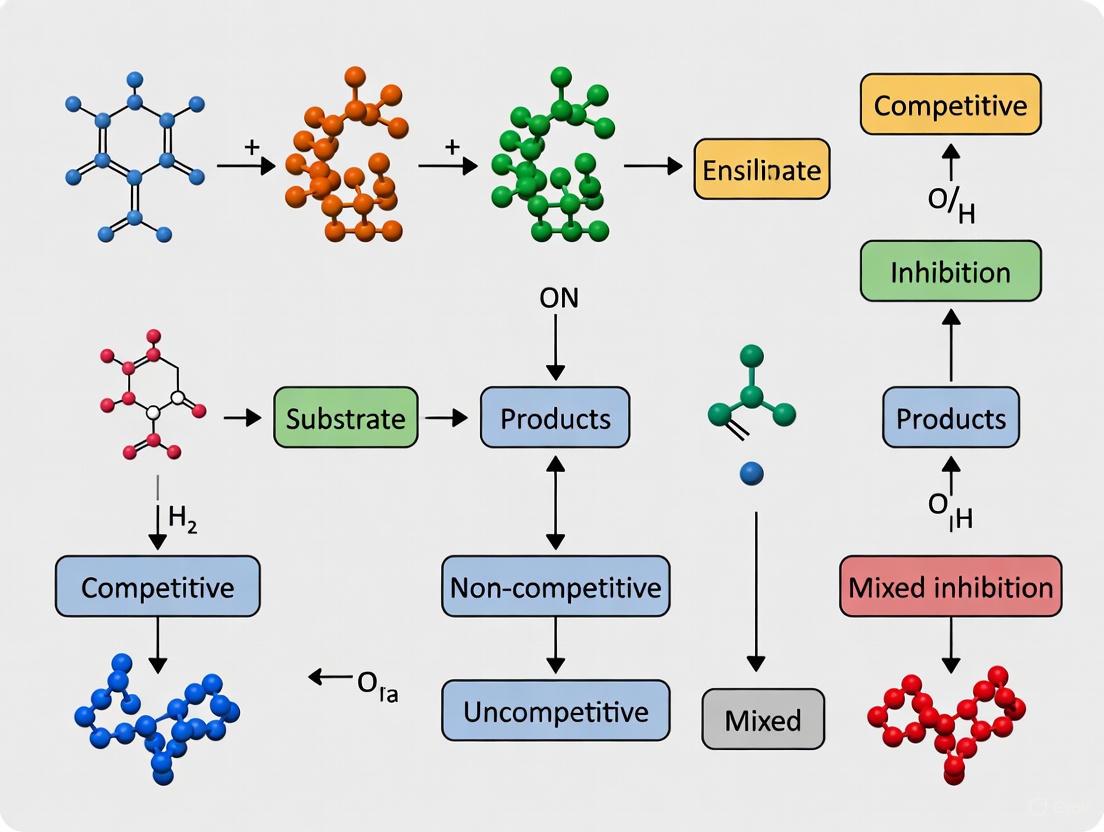
Enzyme inhibition analysis is essential in drug development, necessitating precise estimation of inhibition constants for predicting drug-drug interactions and therapeutic efficacy [8]. The three primary modes of reversible inhibition—competitive, uncompetitive, and mixed—are characterized by distinct mechanisms and kinetic signatures:

• Competitive inhibition: Inhibitor binds exclusively to the free enzyme (E), competing directly with the substrate. Increases apparent Km without affecting Vmax.
• Uncompetitive inhibition: Inhibitor binds only to the enzyme-substrate complex (ES). Decreases both apparent Km and Vmax.
• Mixed inhibition: Inhibitor can bind to both E and ES, but with different affinities. Affects both Km and Vmax values [8].

The initial velocity in the presence of a mixed inhibitor can be described by the equation:

v = (Vmax [S]) / [Km(1 + [I]/Kic) + S]

where Kic and Kiu represent the inhibition constants for binding to the free enzyme and enzyme-substrate complex, respectively [8]. The relative magnitude of these two inhibition constants determines the mechanistic classification of the inhibitor.

Advanced Concepts in Inhibition

Recent research has introduced sophisticated inhibition strategies, including differential inhibition, which targets enzymes capable of acting on multiple substrates selectively [9]. Differential inhibitors (DIs) represent a promising approach for enzymes like aldose reductase, which metabolizes both hydrophilic aldoses (implicated in diabetic complications) and hydrophobic aldehydes (involved in detoxification) [9]. By selectively inhibiting only one catalytic pathway, DIs offer enhanced specificity with reduced off-target effects. In 2025, researchers further advanced inhibition analysis with "50-BOA" (ICâ‚…â‚€-Based Optimal Approach), demonstrating that precise estimation of inhibition constants is possible using a single inhibitor concentration greater than the ICâ‚…â‚€ value, substantially reducing experimental requirements while maintaining accuracy [8].

Diagram 1: Enzyme Inhibition Mechanisms and Effects

Experimental Protocols and Methodological Advances

Standard Protocol for Determining Kinetic Parameters

The reliable determination of Michaelis-Menten parameters requires careful experimental design and execution. The following protocol outlines best practices for initial rate measurements:

• Reaction Conditions: Conduct assays under optimal pH, temperature, and ionic strength conditions using appropriate buffer systems. Include any necessary cofactors or activators.

• Initial Rate Measurements: Measure initial velocities (vâ‚€) under conditions where product formation is linear with time and reverse reactions are negligible. Use enzyme concentrations that yield detectable product formation while maintaining [S] >> [E] conditions.

• Substrate Concentration Range: Employ a substrate concentration range that brackets the Km value, typically from 0.2Km to 5Km. Include a minimum of 8-10 different substrate concentrations for reliable parameter estimation.

• Data Collection: Measure initial rates in duplicate or triplicate for each substrate concentration. Include controls without enzyme and without substrate.

• Parameter Estimation: Fit the Michaelis-Menten equation directly to the untransformed v versus [S] data using nonlinear regression algorithms. Avoid linear transformations like Lineweaver-Burk plots, which can distort error distribution and give misleading results [1].

Ultra-High-Throughput Kinetic Methodologies

Recent technological advances have dramatically increased the scale of kinetic measurements. Methodologies like DOMEK (mRNA-display-based one-shot measurement of enzymatic kinetics) enable quantitative determination of kcat/Km values for hundreds of thousands of substrates in parallel [10]. This approach combines mRNA display with next-generation sequencing to profile substrate specificity landscapes of promiscuous enzymes, such as post-translational modification enzymes, with unprecedented throughput. The experimental pipeline involves:

• Library Preparation: Generation of diverse peptide libraries via mRNA display (>10¹² unique sequences)
• Enzymatic Time Courses: Incubation of enzyme with peptide library across multiple time points
• Product Quantification: NGS-based measurement of substrate conversion yields
• Data Analysis: Fitting of progress curves to extract kcat/Km values for individual substrates [10]

Such high-throughput approaches are transforming enzymology from qualitative substrate identification to quantitative landscape mapping, enabling predictive models of enzyme specificity and mechanism.

Diagram 2: DOMEK High-Throughput Kinetic Screening

The Scientist's Toolkit: Essential Reagents and Materials

Table 3: Research Reagent Solutions for Enzyme Kinetics Studies

Reagent/Material	Function/Application	Technical Considerations
Recombinant Enzymes	Catalytic component of reactions	Purified to homogeneity; concentration accurately determined via absorbance or activity assays
Synthetic Peptide Substrates	Enzyme substrates for specificity profiling	Custom-synthesized with >95% purity; concentrations verified by amino acid analysis
Cofactors (NAD(P)H, ATP, etc.)	Essential reaction components for many enzymes	Freshly prepared solutions; concentration stability verified spectrophotometrically
Coupled Assay Systems	Continuous monitoring of product formation	Include excess coupling enzymes; ensure non-rate-limiting conditions
mRNA Display Libraries	Ultra-high-throughput substrate screening	Library complexity >10¹² sequences; quality control via NGS [10]
Inhibitor Compounds	Mechanism and inhibition constant determination	High-purity compounds dissolved in appropriate solvents with vehicle controls
Neoprocurcumenol	Neoprocurcumenol, CAS:102130-91-6, MF:C15H22O2, MW:234.33 g/mol	Chemical Reagent
Istamycin Y0	Istamycin Y0, MF:C14H30N4O4, MW:318.41 g/mol	Chemical Reagent

Michaelis-Menten kinetics continues to provide an essential foundation for understanding enzyme catalysis more than a century after its initial formulation. While the basic principles remain unchanged, modern research has expanded this framework to address increasingly complex biological questions. Current frontiers include the development of ultra-high-throughput screening methods like DOMEK that can simultaneously quantify kinetic parameters for hundreds of thousands of substrates [10], the integration of structural data with kinetic parameters through resources like SKiD [7], and the refinement of inhibition analysis techniques that reduce experimental burden while improving precision [8]. As these methodologies continue to evolve, they will further enhance our ability to engineer enzymes with tailored properties, design more specific therapeutic inhibitors, and predict metabolic behaviors in complex biological systems. For researchers and drug development professionals, mastery of both the fundamental principles and contemporary advancements in enzyme kinetics remains indispensable for innovation in biochemistry, biotechnology, and pharmaceutical sciences.

Enzyme inhibition analysis is a cornerstone of enzymology and drug discovery, providing critical insights into the regulation of biochemical pathways and the mechanism of action of therapeutic compounds. Reversible inhibition, characterized by non-covalent interactions between the inhibitor and enzyme, allows for equilibrium between the enzyme and inhibitory drug [11] [12]. Understanding these mechanisms is essential for predicting drug interactions, designing targeted therapies, and elucidating metabolic control systems in living organisms. The three primary models of reversible inhibition—competitive, non-competitive, and uncompetitive—are distinguished by their specific binding mechanisms and resultant effects on enzyme kinetic parameters [13]. These inhibition patterns not only reveal the nature of enzyme-inhibitor interactions but also have profound implications for drug efficacy and physiological function.

In drug development, enzyme inhibitors constitute a significant proportion of therapeutic agents, as many drugs function by specifically inhibiting enzymes involved in disease processes [13]. The screening and characterization of these inhibitors through mechanism of action (MOA) studies provide the foundation for structure-activity relationship (SAR) analyses, which guide the optimization of drug candidates for enhanced potency, selectivity, and pharmacological properties [13]. Furthermore, the type of reversible inhibition displayed by a compound determines its behavior under physiological conditions, particularly in the presence of varying substrate concentrations, which directly impacts its therapeutic potential and clinical management strategies [8].

Competitive Inhibition

Mechanism and Binding Characteristics

Competitive inhibition occurs when an inhibitor competes with the substrate for binding to the active site of the enzyme [14]. The inhibitor is typically a structural analog of the substrate, resembling the natural substrate closely enough to bind to the active site but differing in that it cannot undergo catalysis [11] [15]. This binding results in the formation of an enzyme-inhibitor (EI) complex that is catalytically inactive. The fundamental characteristic of competitive inhibition is that the inhibitor binds exclusively to the free enzyme (E) and cannot bind to the enzyme-substrate (ES) complex, making the binding of substrate and inhibitor mutually exclusive events [13] [14].

The reversibility of competitive inhibition means that the inhibitor can dissociate from the enzyme, allowing substrate binding to occur. Consequently, the inhibitory effect can be overcome by increasing the concentration of substrate, as the higher substrate concentration effectively outcompetes the inhibitor for binding to the active site [11] [14]. This property has significant implications for drug design and therapeutic applications, as the efficacy of competitive inhibitors can be influenced by the endogenous concentration of the natural substrate in physiological conditions.

Kinetic Parameters and Graphical Analysis

Competitive inhibition produces distinctive effects on the Michaelis-Menten kinetic parameters of an enzyme. The presence of a competitive inhibitor increases the apparent Michaelis constant (Kₘ) while leaving the maximal reaction velocity (Vₘₐₓ) unchanged [13] [14]. The increase in apparent Kₘ occurs because a higher substrate concentration is required to achieve half-maximal velocity in the presence of the inhibitor, reflecting reduced apparent affinity of the enzyme for its substrate [11].

The Lineweaver-Burk double reciprocal plot provides a characteristic pattern for competitive inhibition. The plots show a series of lines that intersect on the y-axis, indicating that Vₘₐₓ remains constant while the slope (Kₘ/Vₘₐₓ) and x-intercept (-1/Kₘ) change with increasing inhibitor concentration [16] [14]. The inhibitor constant (Kᵢ), which represents the dissociation constant of the enzyme-inhibitor complex, can be determined from secondary plots of the apparent Kₘ or the slopes of the Lineweaver-Burk lines versus inhibitor concentration [13].

The velocity equation for an enzyme reaction in the presence of a competitive inhibitor is modified as follows:

v₀ = (Vₘₐₓ × [S₀]) / (Kₘ × (1 + [I₀]/Kᵢ) + [S₀])

Research and Clinical Applications

Competitive inhibitors have significant therapeutic applications, with many drugs functioning through this mechanism. Methotrexate, an antineoplastic agent, is a classic example of a competitive inhibitor that structurally resembles folic acid and competitively inhibits dihydrofolate reductase, blocking nucleotide synthesis and cell division in rapidly dividing cancer cells [11] [14]. Similarly, the HIV protease inhibitor ritonavir competes with the viral protein substrate for binding to the active site of the HIV protease enzyme [14].

In clinical toxicology, competitive inhibition provides life-saving interventions, as demonstrated in methanol poisoning treatment. Methanol is metabolized by alcohol dehydrogenase to toxic formaldehyde, and treatment involves administering either ethanol or fomepizole, which compete with methanol for the enzyme's active site, preventing the formation of toxic metabolites [14]. Penicillin represents another example, acting as a competitive inhibitor that blocks the active site of bacterial enzymes involved in cell wall synthesis [15].

Table 1: Kinetic Parameters for Competitive Inhibition

Parameter	Effect of Competitive Inhibitor	Theoretical Basis
Vₘₐₓ	Unchanged	At infinite substrate concentration, inhibitor is completely outcompeted
Kₘ	Increases	Higher substrate concentration required to achieve half-maximal velocity
Káµ¢	Dissociation constant for EI complex	Measure of inhibitor affinity for enzyme
Lineweaver-Burk Pattern	Lines intersecting on y-axis	Confirms unchanged Vₘₐₓ with increasing Kₘ

Figure 1: Competitive Inhibition Mechanism - The inhibitor (I) competes with substrate (S) for binding to the active site of the enzyme (E), forming an enzyme-inhibitor complex (EI) that cannot proceed to product formation.

Non-competitive Inhibition

Mechanism and Binding Characteristics

Non-competitive inhibition is characterized by an inhibitor that binds to an allosteric site on the enzyme, distinct from the active site where substrate binding occurs [16] [12]. Unlike competitive inhibitors, non-competitive inhibitors can bind to both the free enzyme (E) and the enzyme-substrate complex (ES) with equal affinity, forming either an enzyme-inhibitor (EI) complex or an enzyme-substrate-inhibitor (ESI) complex [13] [16]. The binding of the non-competitive inhibitor induces conformational changes in the enzyme structure that diminish catalytic activity without affecting substrate binding [16].

The mechanism of non-competitive inhibition does not involve competition between substrate and inhibitor for the same binding site, which means that increasing substrate concentration cannot overcome the inhibition [12]. The ESI complex is typically catalytically inactive or has significantly reduced activity, preventing product formation even when substrate is bound to the enzyme. This allosteric regulation represents a fundamental mechanism for controlling metabolic pathways in physiological systems [16].

Kinetic Parameters and Graphical Analysis

In non-competitive inhibition, the apparent Vₘₐₓ is decreased while the Kₘ value remains unchanged [16] [17]. The reduction in Vₘₐₓ occurs because the inhibitor effectively reduces the concentration of functional enzyme, regardless of substrate concentration. The unchanged Kₘ indicates that the enzyme's affinity for its substrate is not affected, as the substrate can still bind to the enzyme with the same affinity even when the inhibitor is bound at the allosteric site [16].

The Lineweaver-Burk plot for non-competitive inhibition shows a series of lines that intersect on the x-axis, indicating constant Kₘ with decreasing Vₘₐₓ as inhibitor concentration increases [16]. The inhibitor constant Kᵢ can be determined from secondary plots of 1/Vₘₐₓ or the slopes of the Lineweaver-Burk plots versus inhibitor concentration [13]. For simple linear non-competitive inhibition, Kᵢ represents the inhibitor concentration that halves the value of Vₘₐₓ [13].

The velocity equation for non-competitive inhibition is expressed as:

v₀ = (Vₘₐₓ × [S₀]) / ((Kₘ + [S₀]) × (1 + [I₀]/Kᵢ))

Research and Clinical Applications

Non-competitive inhibition plays crucial roles in metabolic regulation and toxicology. In metabolic pathways, feedback inhibition often operates through non-competitive mechanisms, where end products of pathways inhibit earlier enzymes to prevent overproduction [16]. For example, glucose-6-phosphate acts as a non-competitive inhibitor of hexokinase in the brain, shutting down glucose metabolism when sufficient product has accumulated [16]. Similarly, ATP and alanine function as non-competitive inhibitors of pyruvate kinase, the final enzyme in glycolysis, providing regulatory control of energy production [16].

In clinical contexts, cyanide poisoning represents a dramatic example of non-competitive inhibition, where cyanide binds to cytochrome c oxidase in the electron transport chain, disrupting cellular respiration and ATP production [16]. Heavy metals such as mercury, cadmium, and lead also exhibit toxicity through non-competitive inhibition of various essential enzymes [16]. From a therapeutic perspective, research continues to explore non-competitive inhibitors for conditions like type 2 diabetes, where compounds such as Rosha grass components act as non-competitive inhibitors of intestinal alpha-glucosidase, helping to manage postprandial blood glucose levels [16].

Table 2: Kinetic Parameters for Non-competitive Inhibition

Parameter	Effect of Non-competitive Inhibitor	Theoretical Basis
Vₘₐₓ	Decreased	Functional enzyme concentration reduced
Kₘ	Unchanged	Substrate binding affinity unaffected
Káµ¢	Dissociation constant for EI and ESI complexes	Measure of inhibitor affinity
Lineweaver-Burk Pattern	Lines intersecting on x-axis	Confirms unchanged Kₘ with decreasing Vₘₐₓ

Figure 2: Non-competitive Inhibition Mechanism - The inhibitor (I) binds to an allosteric site on both the free enzyme (E) and the enzyme-substrate complex (ES), forming inactive EI and ESI complexes.

Uncompetitive Inhibition

Mechanism and Binding Characteristics

Uncompetitive inhibition represents a less common but mechanistically distinct form of enzyme inhibition where the inhibitor binds exclusively to the enzyme-substrate complex (ES) rather than to the free enzyme [13] [18]. This binding results in the formation of an enzyme-substrate-inhibitor (ESI) complex that is catalytically inactive or has significantly reduced activity. A key characteristic of uncompetitive inhibition is that the inhibitor binding site is typically not available on the free enzyme but becomes exposed only after substrate binding induces a conformational change in the enzyme structure [18].

This sequential binding mechanism means that uncompetitive inhibitors do not compete with substrates for binding, and increasing substrate concentration does not reverse the inhibition but rather enhances it [13] [18]. This paradoxical behavior occurs because higher substrate concentrations lead to more ES complex formation, which in turn provides more target for the uncompetitive inhibitor to bind. The unique properties of uncompetitive inhibition make it particularly significant in physiological regulation and drug design, especially for multi-substrate enzyme systems [18].

Kinetic Parameters and Graphical Analysis

In uncompetitive inhibition, both Vₘₐₓ and Kₘ are decreased by the same factor (1 + [I]/Kᵢ) [13] [18]. The reduction in Vₘₐₓ occurs because the formation of the ESI complex removes active enzyme from the catalytic cycle. The decrease in Kₘ appears counterintuitive but results from the inhibitor binding to and stabilizing the ES complex, effectively increasing the enzyme's apparent affinity for the substrate by reducing the dissociation of substrate from the complex [18].

The Lineweaver-Burk plot for uncompetitive inhibition shows a series of parallel lines, with both the y-intercept (1/Vₘₐₓ) and x-intercept (-1/Kₘ) increasing with higher inhibitor concentrations while the slope (Kₘ/Vₘₐₓ) remains unchanged [18]. The inhibitor constant Kᵢ (often denoted as Kᵢᵢ to specify intercept effects) represents the dissociation constant for the ESI complex and can be determined from secondary plots of the apparent Vₘₐₓ or 1/Vₘₐₓ versus inhibitor concentration [13].

The velocity equation for uncompetitive inhibition is expressed as:

v₀ = (Vₘₐₓ × [S₀]) / (Kₘ + [S₀] × (1 + [I₀]/Kᵢ))

Research and Clinical Applications

Uncompetitive inhibition, while relatively rare compared to other forms of inhibition, offers unique advantages in therapeutic applications. Because uncompetitive inhibitors bind only to the enzyme-substrate complex, they selectively target actively catalyzing enzymes, potentially reducing off-target effects [18]. This specificity makes them particularly attractive for drug development against enzymes that exist in multiple states or conformations.

In clinical contexts, the management of uncompetitive inhibition presents distinct challenges. Unlike competitive inhibition where dose adjustments can help mitigate risks, therapeutic interventions are less effective for uncompetitive inhibitors, making clinical management more complicated [8]. This underscores the importance of identifying inhibition mechanisms during drug development to anticipate potential clinical behaviors and design appropriate dosing strategies.

Uncompetitive inhibition is more commonly observed in multi-reactant enzyme systems than single-substrate reactions, making it particularly relevant for complex metabolic pathways and signaling cascades [18]. The study of uncompetitive inhibition continues to provide insights into enzyme mechanisms and opportunities for designing highly specific therapeutic agents with reduced side-effect profiles.

Table 3: Kinetic Parameters for Uncompetitive Inhibition

Parameter	Effect of Uncompetitive Inhibitor	Theoretical Basis
Vₘₐₓ	Decreased	ES complex diverted to inactive ESI complex
Kₘ	Decreased	ES complex stabilized by inhibitor binding
Káµ¢	Dissociation constant for ESI complex	Measure of inhibitor affinity for ES complex
Lineweaver-Burk Pattern	Parallel lines	Proportional decrease in both Vₘₐₓ and Kₘ

Figure 3: Uncompetitive Inhibition Mechanism - The inhibitor (I) binds exclusively to the enzyme-substrate complex (ES), forming an inactive ESI complex without binding to free enzyme.

Experimental Protocols and Methodologies

Classical Steady-State Inhibition Analysis

The classical approach to enzyme inhibition analysis involves measuring initial reaction velocities under steady-state conditions across a range of substrate and inhibitor concentrations [13]. The fundamental protocol begins with determining enzyme activity in the absence of inhibitor to establish baseline kinetic parameters (Vₘₐₓ and Kₘ). Subsequently, reactions are conducted with varying concentrations of inhibitor, typically spanning several orders of magnitude around the expected inhibition constant [13]. For each inhibitor concentration, initial velocities are measured at multiple substrate concentrations, usually ranging from 0.2×Kₘ to 5×Kₘ to adequately characterize the inhibition pattern [13] [8].

Data collection follows a systematic matrix design where each combination of substrate and inhibitor concentrations is tested in replicate to ensure statistical reliability. The reaction conditions—including pH, temperature, ionic strength, and cofactor concentrations—must be rigorously controlled and optimized for the specific enzyme system under investigation [13]. Continuous assays employing spectrophotometric, fluorometric, or radiometric detection methods are preferred when possible, as they provide more data points for accurate velocity determination compared to endpoint assays [13].

ICâ‚…â‚€-Based Optimal Approach (50-BOA)

Recent advancements in inhibition analysis have introduced more efficient experimental designs that reduce resource requirements while maintaining precision. The ICâ‚…â‚€-Based Optimal Approach (50-BOA) represents a significant innovation that enables precise estimation of inhibition constants using a single inhibitor concentration greater than the half-maximal inhibitory concentration (ICâ‚…â‚€) [8]. This method substantially reduces the number of required experiments by more than 75% compared to conventional approaches while ensuring accuracy and precision [8].

The 50-BOA protocol begins with prior estimation of IC₅₀ from percentage control activity data across various inhibitor concentrations at a single substrate concentration, typically equal to Kₘ [8]. Subsequently, comprehensive initial velocity measurements are performed using a single inhibitor concentration greater than the determined IC₅₀ value across the full range of substrate concentrations [8]. By incorporating the fundamental relationship between IC₅₀ and inhibition constants into the fitting process, this approach achieves comparable precision to traditional methods with significantly reduced experimental burden [8].

The mathematical foundation of 50-BOA relies on the error landscape analysis of inhibition constant estimations, which revealed that data obtained with low inhibitor concentrations provide minimal information for constant estimation, while high inhibitor concentrations dramatically reduce estimation error [8]. This approach is particularly valuable in drug discovery settings where high-throughput screening of multiple compounds is necessary, as it enables rapid characterization of inhibition mechanisms and constants without compromising data quality.

Data Analysis and Validation

Analysis of inhibition data typically begins with visualization using Lineweaver-Burk plots to identify the inhibition pattern, followed by nonlinear regression fitting to the appropriate velocity equation to determine kinetic parameters and inhibition constants [13]. Statistical validation includes assessment of goodness-of-fit metrics, residual analysis, and determination of confidence intervals for estimated parameters [13] [8]. For mixed inhibition models involving two inhibition constants, additional validation through global fitting across multiple inhibitor concentrations is essential to ensure parameter identifiability and prevent false reporting of inhibition types [8].

Secondary plots provide crucial validation of inhibition constants and mechanisms. For competitive inhibition, plots of apparent Kₘ versus inhibitor concentration should yield linear relationships with x-intercepts of -Kᵢ [13]. For non-competitive inhibition, plots of 1/Vₘₐₓ versus inhibitor concentration provide Kᵢ values from x-intercepts [13]. Dixon plots (1/v versus [I]) represent an alternative method for determining Kᵢ values, with all inhibition types yielding linear relationships that intersect at -Kᵢ [13].

Table 4: Experimental Design for Comprehensive Inhibition Analysis

Experimental Condition	Traditional Approach	50-BOA Approach	Purpose
Substrate Concentrations	0.2×Kₘ, Kₘ, 5×Kₘ	Full range (0.2×Kₘ to 5×Kₘ)	Characterize substrate dependence
Inhibitor Concentrations	0, ⅓×IC₅₀, IC₅₀, 3×IC₅₀	Single concentration > IC₅₀	Determine inhibitor potency
ICâ‚…â‚€ Determination	Required for design	Required for design	Establish inhibitor potency range
Data Points Required	12-16 combinations	3-5 substrate concentrations	Balance precision and efficiency

Figure 4: Experimental Workflow for Inhibition Studies - Comparison of traditional and 50-BOA approaches for enzyme inhibition analysis, highlighting significant reduction in experimental requirements with the optimized method.

The Scientist's Toolkit: Essential Research Reagents and Materials

Successful investigation of reversible inhibition mechanisms requires carefully selected reagents and specialized materials designed to maintain enzyme stability, ensure measurement precision, and enable accurate detection of reaction products. The following essential components represent the core toolkit for researchers conducting enzyme inhibition studies.

Table 5: Essential Research Reagents for Enzyme Inhibition Studies

Reagent/Material	Specification	Function in Inhibition Studies
Purified Enzyme	High purity (>95%), known concentration	Primary target for inhibition studies; must have well-characterized specific activity
Natural Substrate	High purity, structurally characterized	Native reactant for establishing baseline kinetics and inhibition patterns
Inhibitor Compounds	>95% purity, solubilized in appropriate solvent	Test compounds for mechanism elucidation; require precise concentration verification
Assay Buffer System	pH-optimized, appropriate ionic strength	Maintains enzyme stability and activity; prevents pH artifacts in inhibition measurements
Cofactors/Prosthetic Groups	Enzyme-specific (NAD/H, metal ions, etc.)	Essential for enzymes requiring cofactors; concentration must be saturating
Detection Reagents	Spectrophotometric/fluorometric substrates	Enable monitoring of reaction progress; must have appropriate sensitivity and dynamic range
Positive Control Inhibitors	Well-characterized inhibition mechanism	Validation of experimental system and comparison of inhibitor potency
Stopping Reagents	Acid, base, or specific quenchers	Terminate reactions at precise time points for endpoint assays
Angustifoline	Angustifoline, MF:C14H22N2O, MW:234.34 g/mol	Chemical Reagent
Mycinamicin VII	Mycinamicin VII|Macrolide Antibiotic|RUO	Mycinamicin VII is a 16-membered macrolide antibiotic for antimicrobial mechanism research. This product is For Research Use Only. Not for human or veterinary use.

The selection of appropriate buffer systems deserves particular emphasis, as pH can significantly influence enzyme activity and inhibitor binding [13]. Buffers should be chosen based on their pKₐ values relative to the optimal pH for enzyme activity and their lack of specific ion effects that might alter enzyme conformation or inhibitor interactions. For metal-dependent enzymes, chelating agents may be incorporated into control experiments to verify metal requirement, but must be excluded from main inhibition studies to prevent confounding effects [13].

Detection methods must be optimized for the specific enzyme system under investigation. Continuous spectrophotometric or fluorometric assays are preferred when possible, as they provide multiple data points from single reactions and allow direct verification of linear initial velocity conditions [13]. For endpoint assays, the linear range of the assay must be thoroughly characterized, and reaction times adjusted to ensure that substrate depletion remains below 10% to maintain steady-state conditions [13]. Recent advancements in detection technologies, including coupled enzyme systems and high-throughput compatible methods, have expanded the toolbox available for comprehensive inhibition studies.

Enzyme kinetics provides a fundamental framework for understanding catalytic efficiency and enzyme-substrate interactions in biochemical systems. The parameters ( KM ), ( V{max} ), and ( k_{cat} ) offer critical insights into enzyme function, enabling researchers to quantify catalytic proficiency, substrate affinity, and turnover capacity. Within drug development and metabolic engineering, these parameters inform inhibitor design, pathway regulation, and therapeutic targeting. This technical guide examines the theoretical foundation, experimental determination, and biochemical significance of these core kinetic parameters, contextualized within contemporary enzyme research and industrial applications.

Enzyme kinetics is the study of reaction rates catalyzed by enzymes and the conditions affecting these rates [19]. This discipline reveals catalytic mechanisms, regulatory control points, and potential therapeutic intervention strategies [19]. The quantitative analysis of enzyme behavior allows researchers to predict metabolic flux, identify rate-limiting steps in biochemical pathways, and design effective inhibitors for pharmaceutical applications [20].

The Michaelis-Menten model, first introduced in 1913, remains the cornerstone for understanding single-substrate enzyme kinetics [21] [22]. This model describes how reaction velocity varies with substrate concentration, characterized by a hyperbolic relationship that approaches a maximum velocity (( V_{max} )) as substrate concentration increases [23] [24]. The model relies on several key assumptions: that the reaction occurs under steady-state conditions, enzyme concentration remains constant, and only initial rates are measured before significant product accumulation occurs [19] [25].

Fundamental Kinetic Parameters

The Michaelis Constant (( K_M ))

The Michaelis constant (( KM )) is defined as the substrate concentration at which the reaction rate is half of ( V{max} ) [24] [22]. Mathematically, ( KM ) is expressed as ( KM = \frac{k{-1} + k{cat}}{k1} ), where ( k{-1} ) and ( k1 ) are the rate constants for the dissociation and formation of the enzyme-substrate complex, respectively, and ( k{cat} ) is the catalytic rate constant [19]. In the specific case where ( k{cat} ) is much smaller than ( k{-1} ), ( KM ) approximates the dissociation constant (( KD )) of the enzyme-substrate complex, thus providing a direct measure of substrate affinity [19]. A lower ( K_M ) value indicates higher enzyme-substrate affinity, meaning the enzyme can achieve half-maximal velocity at lower substrate concentrations [26] [22].

Maximum Velocity (( V_{max} ))

( V{max} ) represents the maximum reaction rate achieved when an enzyme is fully saturated with substrate [23] [24]. At this point, all enzyme active sites are occupied, and the reaction rate depends solely on the intrinsic turnover capacity of the enzyme [19]. ( V{max} ) is directly proportional to enzyme concentration, as expressed by the relationship ( V{max} = k{cat} \cdot [E]{tot} ), where ( [E]{tot} ) is the total enzyme concentration [19]. This proportional relationship distinguishes ( V{max} ) from ( KM ), the latter being independent of enzyme concentration [24].

Turnover Number (( k_{cat} ))

The turnover number (( k{cat} )), also known as the turnover rate or turnover frequency, quantifies the maximum number of substrate molecules converted to product per enzyme molecule per unit time [24] [27]. Calculated as ( k{cat} = \frac{V{max}}{[E]{tot}} ), this parameter provides a measure of catalytic efficiency independent of enzyme concentration [24]. Turnover numbers vary dramatically between enzymes, from approximately 1 per second for tyrosinase to over 600,000 per second for carbonic anhydrase (Table 1) [27]. This remarkable variation reflects evolutionary adaptation to specific physiological demands and substrate characteristics.

Catalytic Efficiency (( k{cat}/KM ))

The ratio ( k{cat}/KM ) represents the catalytic efficiency of an enzyme, combining both substrate binding affinity (( KM )) and catalytic rate (( k{cat} )) into a single parameter [26]. This ratio has dimensions of a second-order rate constant (M⁻¹s⁻¹) and describes the enzyme's effectiveness at low substrate concentrations [26]. A higher ( k{cat}/KM ) value indicates greater catalytic proficiency, with some enzymes approaching the diffusion-controlled limit of approximately 10⁸ to 10⁹ M⁻¹s⁻¹ [26].

Table 1: Representative Turnover Numbers and Kinetic Parameters for Common Enzymes

Enzyme	( k_{cat} ) (s⁻¹)	( K_M ) (mM)	( k{cat}/KM ) (M⁻¹s⁻¹)	Catalytic Efficiency
Carbonic anhydrase	600,000 [27]	~26 [27]	~2.3×10⁷	Extremely high
Catalase	93,000 [27]	-	-	Very high
β-Galactosidase	200 [27]	-	-	Moderate
Chymotrypsin	100 [27]	-	-	Moderate
Tyrosinase	1 [27]	-	-	Low

Experimental Determination of Kinetic Parameters

Initial Rate Measurements and Assay Conditions

Accurate determination of kinetic parameters requires careful measurement of initial reaction rates under conditions where substrate depletion, product inhibition, and enzyme instability are minimized [28] [19]. Enzyme assays should be conducted during the steady-state phase, typically the first few percent of the reaction, where the concentration of the enzyme-substrate complex remains relatively constant [23] [19].

Assay conditions must be carefully controlled, as kinetic parameters are dependent on temperature, pH, ionic strength, and buffer composition [28]. Researchers should ideally use conditions that reflect the enzyme's physiological environment, though this is not always practiced in literature reports [28]. Common pitfalls include using non-physiological substrates for easier detection, inappropriate pH values that shift reaction equilibria, and variable temperatures that complicate comparisons between studies [28].

Figure 1: Workflow for determining enzyme kinetic parameters, highlighting critical experimental considerations.

Data Analysis and Linearization Methods

The Michaelis-Menten equation, ( v0 = \frac{V{max}[S]}{KM + [S]} ), describes the hyperbolic relationship between initial velocity (( v0 )) and substrate concentration ([S]) [19]. While nonlinear regression of the direct plot provides the most accurate parameter estimates, linear transformations such as the Lineweaver-Burk plot (1/vâ‚€ vs. 1/[S]) offer visual insights into enzyme inhibition mechanisms [23]. The Lineweaver-Burk plot yields a straight line with a y-intercept of 1/Vmax and an x-intercept of -1/KM [23].

The Scientist's Toolkit: Essential Research Reagents

Table 2: Key Reagents for Enzyme Kinetic Studies

Reagent/Category	Function & Importance	Technical Considerations
Purified Enzyme	Catalytic entity under investigation; source and purity critical	Specify organism, tissue, isoenzyme; confirm purity and activity; note potential commercial variations [28]
Natural Substrate	Physiological reactant for the enzyme	Preferred for relevance; may present detection challenges [28]
Analog Substrate	Alternative reactant with more easily detectable products	Enables high-throughput screening; verify kinetic behavior matches natural substrate [28]
Appropriate Buffer	Maintains optimal pH and ionic environment	Consider chelating properties, specific ion effects, and physiological relevance [28]
Cofactors/Coenzymes	Essential non-protein components for many enzymes	Required for holenzyme formation; concentration optimization needed [27]
Detection System	Quantifies product formation or substrate depletion	Spectrophotometric, radiometric, or coupled assays; ensure linear range [19]
3-Deoxyaphidicolin	3-Deoxyaphidicolin|DNA Polymerase α Inhibitor	3-Deoxyaphidicolin is a specific eukaryotic DNA synthesis inhibitor for research use only (RUO). It competitively inhibits DNA polymerase alpha. Not for human or veterinary use.
Epithienamycin A	Epithienamycin A|Carbapenem Antibiotic|RUO	Epithienamycin A is a natural β-lactam antibiotic for research of bacterial resistance and novel carbapenems. For Research Use Only. Not for human use.

Biochemical Interpretation and Significance

Physiological Relevance of Kinetic Parameters

In metabolic pathways, enzymes with high catalytic efficiency (( k{cat}/KM )) often operate near diffusion-controlled limits, while those with lower efficiency may serve as regulatory points [20]. The ( KM ) value typically approximates the physiological substrate concentration, allowing enzymes to respond sensitively to changes in metabolite levels [19]. This relationship enables efficient metabolic regulation, as small fluctuations in substrate concentration around the ( KM ) value produce significant changes in reaction rate [19].

Enzyme kinetics also provides crucial insights for understanding metabolic diseases. Abnormal levels of specific metabolites may indicate alterations in the rate-limiting steps of pathways, potentially due to genetic deficiencies, environmental toxins, or pathological conditions [20]. Kinetic analysis can identify which enzyme in a patient's pathway has become newly rate-limiting, informing potential therapeutic strategies [20].

Enzyme Inhibition and Drug Design

Kinetic parameters are essential for characterizing enzyme inhibition mechanisms, which form the basis for many pharmaceutical compounds [22]. Competitive inhibitors increase the apparent ( KM ) without affecting ( V{max} ) by competing with the substrate for the active site [22]. Uncompetitive inhibitors bind exclusively to the enzyme-substrate complex, decreasing both apparent ( KM ) and ( V{max} ) [21]. Non-competitive inhibitors bind to both free enzyme and enzyme-substrate complex, reducing ( V{max} ) while leaving ( KM ) unchanged [21] [22].

Figure 2: Enzyme inhibition mechanisms showing competitive (EI), uncompetitive (ESI), and mixed inhibition pathways.

Advanced Considerations in Enzyme Kinetics

Multi-Substrate Reactions

Many enzymes catalyze reactions involving two or more substrates, requiring more complex kinetic mechanisms [21] [19]. Sequential mechanisms require all substrates to bind before any products are released, with ordered mechanisms specifying a mandatory binding sequence and random mechanisms allowing flexible substrate association [21]. Ping-pong mechanisms involve covalent modification of the enzyme and release of one product before all substrates have bound, characteristic of transaminases and phosphotransferases [21] [19].

Cooperativity and Allosteric Regulation

Enzymes with multiple subunits often display cooperativity, where substrate binding to one active site influences substrate affinity at subsequent sites [25]. Positive cooperativity results in a sigmoidal velocity vs. substrate concentration curve, with the Hill equation modifying the Michaelis-Menten relationship to accommodate this behavior [21]. Allosteric effectors modulate enzyme activity by binding at regulatory sites distinct from the active site, providing crucial metabolic feedback control [28].

The reliability of kinetic parameters depends heavily on experimental conditions and reporting standards [28]. Researchers should critically evaluate literature values for factors such as appropriate assay conditions, initial rate measurements, and physiological relevance [28]. Databases such as BRENDA, SABIO-RK, and STRENDA provide curated kinetic parameters with source references, with STRENDA establishing reporting standards to improve data reliability [28].

The kinetic parameters ( KM ), ( V{max} ), and ( k_{cat} ) provide fundamental insights into enzyme function that extend from basic biochemical understanding to applied pharmaceutical development. Proper determination and interpretation of these parameters requires careful experimental design, appropriate assay conditions, and critical evaluation of results within physiological context. As enzyme kinetics continues to evolve with improved measurement technologies and standardized reporting, these parameters remain essential for elucidating catalytic mechanisms, designing therapeutic interventions, and understanding metabolic regulation in health and disease.

The drug-target residence time model represents a paradigm shift in drug discovery, moving beyond traditional equilibrium affinity measurements to incorporate kinetic parameters that often better predict in vivo efficacy. While classical drug affinity parameters (Kd, Ki, IC50) describe binding potency at equilibrium, drug-target residence time (tR), defined as the reciprocal of the dissociation rate constant (1/koff), provides crucial information about the duration of the drug-target complex [29] [30]. This concept has gained significant attention in recent years as researchers recognize that biological systems are dynamic, with drugs entering and leaving circulation through absorption, distribution, metabolism, and excretion (ADME) processes [31]. The residence time concept acknowledges that a drug is only pharmacologically active when bound to its target, suggesting that prolonged residence time could extend therapeutic effects even after free drug concentrations have declined below effective levels [31].

The fundamental relationship between binding kinetics and residence time can be described through the simple binding mechanism:

Where R represents the receptor, L the ligand (drug), RL the drug-receptor complex, kon the association rate constant, and koff the dissociation rate constant [30]. The equilibrium dissociation constant (Kd) is defined as koff/kon, while the drug-target residence time (tR) equals 1/koff [30]. This review explores the theoretical foundation, experimental evidence, methodological approaches, and ongoing controversies surrounding the drug-target residence time concept, providing researchers with a comprehensive framework for applying these principles in drug discovery.

Theoretical Foundation and Kinetic Principles

Fundamental Kinetic Equations

The mathematical foundation of drug-target residence time begins with the basic equations governing molecular interactions. For the simple one-step binding mechanism described above, the dissociation rate constant (koff) directly determines the stability of the drug-target complex. The probability that a drug-target complex remains intact over time follows an exponential decay function:

Where [RL]t represents the concentration of the drug-target complex at time t, and [RL]0 represents the initial complex concentration [30]. The half-life (t1/2) of the complex is calculated as ln(2)/koff, which approximately equals 0.693/koff [31]. This relationship demonstrates that compounds with slower dissociation rates form more persistent complexes with their targets, potentially leading to longer-lasting pharmacological effects.

The crucial relationship between residence time and overall drug effect emerges when considering the dynamic nature of in vivo systems. Unlike in vitro closed systems where equilibrium measurements predominate, in vivo environments represent open systems where drugs are subject to continuous elimination and distribution [31]. The theoretical benefit of long residence time becomes most apparent when the dissociation rate (koff) is slower than the rate of pharmacokinetic elimination (kelim), potentially allowing target engagement to persist even after systemic drug concentrations have become negligible [29].

Comparative Analysis of Binding Kinetics Parameters

Table 1: Key Parameters in Drug-Target Binding Kinetics

Parameter	Symbol	Definition	Relationship to Efficacy
Association Rate Constant	kon	Rate of complex formation (M⁻¹s⁻¹)	Determines how quickly drug reaches target
Dissociation Rate Constant	koff	Rate of complex breakdown (s⁻¹)	Inversely related to duration of effect
Equilibrium Dissociation Constant	Kd	koff/kon (M)	Measures binding affinity at equilibrium
Drug-Target Residence Time	tR	1/koff (time)	Measures duration of target engagement
Inhibition Constant	Ki	Functional analog of Kd for enzymes	Classical measure of inhibitor potency
IC50	IC50	Concentration for 50% inhibition	Functional potency under specific conditions

Experimental Evidence and Validation Studies

In Vivo Displacement Assay for Target Occupancy

A groundbreaking approach to validating the residence time concept came from the development of an in vivo displacement assay using soluble epoxide hydrolase (sEH) as a model system [31]. This innovative methodology enabled researchers to directly monitor drug-target engagement in living organisms, addressing a critical gap in kinetic pharmacology. The experimental workflow follows these key stages:

• Loading Phase: Administration of a loading compound (Inhibitor A) at concentrations sufficient to achieve near-complete target occupancy (typically ≥100× Ki) [31]

• Clearance Phase: A post-dosing period allowing for systemic clearance of unbound drug molecules through metabolism and excretion

• Displacement Phase: Administration of a high-dose displacement compound (Inhibitor B) that competes for the same binding site

• Detection Phase: Measurement of returning blood levels of the original compound as it is displaced from its target [31]

This methodology demonstrated that the sEH inhibitor TPPU (Ki = 2.5 nM, tR = 28.6 minutes) remained bound to its target in vivo long after free drug concentrations had declined to negligible levels [31]. When the displacement compound TCPU was administered seven days after TPPU dosing, a distinct secondary peak of TPPU appeared in blood measurements, confirming that a substantial amount of drug remained target-bound despite undetectable free circulating concentrations [31]. This provided direct experimental evidence that drug-target residence time significantly influences the duration of target occupancy in vivo.

Relationship Between Residence Time and Pharmacokinetics

The sEH inhibitor study revealed an additional crucial dimension of residence time effects—the impact on drug metabolism rates. Researchers observed that compounds with longer residence times were protected from metabolic degradation, effectively extending their functional half-lives [31]. This phenomenon creates a self-reinforcing cycle where prolonged target binding reduces exposure to metabolic enzymes, which in turn further extends the duration of action.

Table 2: Experimental Parameters for sEH Inhibitors in Residence Time Study

Parameter	TPPU	TCPU
Inhibition Constant (Ki)	2.5 nM	0.92 nM
Residence Time (tR)	28.6 min	23.8 min
Dissociation Half-Life (t1/2)	19.8 min	16.5 min
PK Elimination Half-Life	13.0 h	Not specified
Cmax at Test Dose	456 nM	4114 nM
AUC	8813 nM·h	56254 nM·h

These findings fundamentally challenge the traditional separation between pharmacokinetics (what the body does to the drug) and pharmacodynamics (what the drug does to the body) [31]. Instead, they suggest a complex interplay where binding kinetics influence metabolic fate, which in turn modulates therapeutic effects. This relationship may explain why residence time often correlates better with in vivo efficacy than traditional affinity measurements.

Methodological Advances and Experimental Protocols

Enzyme Inhibition Analysis and the 50-BOA Method

Recent methodological advances have revolutionized the estimation of inhibition parameters, including those relevant to residence time calculations. The novel IC50-Based Optimal Approach (50-BOA) enables precise estimation of inhibition constants using dramatically reduced experimental data [8]. Traditional methods require multiple substrate and inhibitor concentrations, but the 50-BOA demonstrates that accurate, precise estimation can be achieved with a single inhibitor concentration greater than the IC50 value [8].

The 50-BOA protocol follows these essential steps:

• IC50 Determination: Estimate the half-maximal inhibitory concentration using a single substrate concentration (typically at KM) across various inhibitor concentrations [8]

• Single-Concentration Design: Measure initial reaction velocities at three substrate concentrations (0.2KM, KM, and 5KM) with a single inhibitor concentration > IC50 [8]

• Model Fitting: Fit the mixed inhibition model to the data using the relationship between IC50 and inhibition constants to constrain parameter estimation [8]

This approach reduces the required experimental data by >75% while improving precision and accuracy compared to traditional methods [8]. The 50-BOA method is particularly valuable for early drug discovery when compound availability is limited and rapid screening of multiple candidates is essential.

Experimental Workflow for Residence Time Determination

The following diagram illustrates the integrated experimental workflow for determining drug-target residence time and its relationship to in vivo efficacy:

Critical Perspectives and Controversies

Despite encouraging experimental evidence, the drug-target residence time concept faces substantial theoretical and practical challenges. A significant criticism concerns the mathematical foundation of the claim that prolonged residence time can cause pharmacodynamic effects to outlast pharmacokinetic exposure [29] [30]. Careful analysis reveals that for this prolongation to occur, the binding dissociation rate must be slower than the pharmacokinetic elimination rate [29]. However, data from numerous drugs and drug candidates show the opposite pattern—elimination rates are typically slower than dissociation rates [29]. This discrepancy severely limits the practical utility of residence time for predicting duration of action in vivo.

Another serious concern involves the equivalence between residence time and affinity. Critics argue that pursuing long residence time is fundamentally similar to pursuing high affinity, since koff contributes directly to both parameters [30]. In most practical cases, compounds with improved residence time also show enhanced affinity, making it difficult to isolate the unique contribution of residence time to efficacy [30]. Additionally, the residence time literature often emphasizes koff while neglecting kon, despite the importance of association rates for achieving rapid target engagement [30].

The relationship between different inhibition types and their kinetic parameters further complicates the residence time concept. Competitive inhibitors generally produce more pronounced drug-drug interactions than non-competitive inhibitors with the same Ki value [32]. Similarly, complete inhibitors typically cause more significant interactions than partial inhibitors [32]. These observations highlight that the mechanistic details of inhibition significantly influence in vivo effects beyond what residence time alone can capture.

Research Reagent Solutions and Technical Tools

Table 3: Essential Research Reagents and Tools for Residence Time Studies

Reagent/Tool	Function/Application	Example/Specifications
sEH Inhibitor Library	Comprehensive compound collection for residence time studies	~3000 compounds with diverse potency, physical properties, and PK parameters [31]
Recombinant sEH Enzymes	Well-characterized enzyme system for kinetic studies	Highly pure recombinant enzymes from multiple species [31]
LC/MS-MS Systems	Sensitive quantification of drug concentrations in biological matrices	Limit of quantification ≤0.5 nM for precise blood and tissue measurements [31]
50-BOA Software Package	Automated estimation of inhibition constants	User-friendly MATLAB and R packages implementing IC50-based optimal approach [8]
In Vivo Displacement Assay Components	Complete system for measuring target occupancy in live animals	Includes loading compounds, displacement compounds, and analytical methods [31]

The drug-target residence time concept represents both an important advance and a subject of ongoing debate in drug discovery. While substantial evidence confirms that binding kinetics influence target engagement duration and metabolic protection [31], theoretical concerns about the overemphasis on koff separate from overall affinity remain unresolved [29] [30]. The most productive path forward likely involves integrated optimization of multiple parameters rather than singular focus on residence time.

Future research should prioritize developing more sophisticated models that simultaneously incorporate binding kinetics, pharmacokinetics, and tissue distribution. The continued refinement of experimental methods like the 50-BOA approach [8] and in vivo displacement assays [31] will provide increasingly precise data to validate and refine these models. Additionally, expanding residence time studies beyond soluble epoxide hydrolase to diverse target classes will clarify the generalizability of current findings.

For drug discovery practitioners, the current evidence supports measuring binding kinetics as a routine component of compound characterization while maintaining a balanced perspective on their interpretation. Residence time data provide valuable insights that complement rather than replace traditional affinity measurements, together enabling more informed decisions in the quest for efficacious therapeutics.

Evolution from IC50 to Kinetic Parameters in Modern Drug Discovery

The half-maximal inhibitory concentration (IC₅₀) has long served as a foundational metric in drug discovery for ranking compound potency. However, this single-parameter approach provides an incomplete picture of inhibitor-enzyme interactions, failing to distinguish between binding affinity and efficiency. Contemporary drug discovery has increasingly shifted toward full kinetic characterization using parameters such as the inhibition constant (Kᵢ) and covalent modification rate constants (k₅ and k₆) that offer mechanistic insights and superior predictive value for in vivo performance. This technical guide examines innovative methodologies—including implicit equation modeling, EPIC-CoRe, and IC₅₀-Based Optimal Approach (50-BOA)—that transform time-dependent IC₅₀ data into meaningful kinetic parameters, enabling more reliable candidate selection and optimization in modern pharmaceutical development.

Enzyme inhibition analysis constitutes a critical component of pharmaceutical development, from initial target validation to lead compound optimization. Traditional approaches have heavily relied on IC₅₀ values—the concentration of inhibitor required to reduce enzyme activity by 50% under specific assay conditions. While providing a useful initial potency measure, IC₅₀ represents an apparent value that varies significantly with experimental conditions, including substrate concentration, pre-incubation time, and enzyme levels [33]. This limitation substantially compromises its utility for comparing inhibitor potency across different laboratories and assay formats.

The evolution toward kinetic parameter determination addresses fundamental shortcomings of IC₅₀-based assessment. Kinetic parameters such as Kᵢ (inhibition constant) and k₍ᵢ₎ (rate constants) provide mechanism-independent constants that quantify the true binding affinity between inhibitor and enzyme target [34]. For reversible covalent inhibitors, which establish their covalent modification equilibrium slowly, additional parameters including the covalent modification rate constants (k₅ and k₆) are essential for understanding both binding and reactivity [35]. These parameters enable accurate ranking of drug candidates by distinguishing compounds with rapid binding from those with prolonged target residence times—a critical differentiator for in vivo efficacy.

Theoretical Foundation: From ICâ‚…â‚€ to Meaningful Kinetic Parameters

Fundamental Kinetic Constants and Their Significance

The transition from ICâ‚…â‚€ to kinetic parameters requires understanding several fundamental constants that define enzyme-inhibitor interactions:

• Káµ¢ (Inhibition Constant): The dissociation constant for the enzyme-inhibitor complex, with lower values indicating tighter binding. Unlike ICâ‚…â‚€, Káµ¢ is a true constant independent of assay conditions [34].
• Kₘ (Michaelis Constant): The substrate concentration at half-maximal enzyme velocity, representing enzyme-substrate affinity [28].
• Vₘₐₓ (Maximum Velocity): The maximum reaction rate when enzyme is fully saturated with substrate [28].
• kâ‚… and k₆: Forward and reverse rate constants for reversible covalent inhibitors, defining the establishment and breakdown of covalent enzyme-inhibitor complexes [35].

For reversible inhibitors, the relationship between IC₅₀ and Kᵢ varies according to inhibition mechanism. In competitive inhibition, the Cheng-Prusoff equation describes this relationship: Kᵢ = IC₅₀ / (1 + [S]/Kₘ), where [S] is substrate concentration and Kₘ is Michaelis constant [34]. This relationship demonstrates the substrate dependence of IC₅₀ values—a fundamental limitation addressed by kinetic parameter determination.

Enzyme Inhibition Mechanisms and Their Kinetic Signatures

Understanding inhibition mechanisms is essential for appropriate experimental design and data interpretation:

• Competitive Inhibition: Inhibitor competes with substrate for binding to the enzyme active site. Characterized by increased apparent Kₘ without effect on Vₘₐₓ [36].
• Uncompetitive Inhibition: Inhibitor binds exclusively to the enzyme-substrate complex. Results in decreased apparent Kₘ and Vₘₐₓ [8].
• Mixed Inhibition: Inhibitor binds to both enzyme and enzyme-substrate complex with different dissociation constants (Káµ¢c and Káµ¢u) [8].

Table 1: Kinetic Signatures of Major Enzyme Inhibition Mechanisms

Inhibition Type	Binding Site	Effect on Apparent Kₘ	Effect on Apparent Vₘₐₓ	Lineweaver-Burk Pattern
Competitive	Enzyme active site	Increases	Unchanged	Intersecting at y-axis
Uncompetitive	Enzyme-substrate complex	Decreases	Decreases	Parallel lines
Mixed	Both enzyme and enzyme-substrate complex	Increases or decreases	Decreases	Intersecting in second quadrant

Modern Methodologies for Kinetic Parameter Estimation

Advanced Mathematical Approaches

Contemporary solutions address the limitations of traditional ICâ‚…â‚€ measurements through sophisticated mathematical modeling:

Implicit Equation Modeling for Reversible Covalent Inhibitors For reversible covalent inhibitors that establish equilibrium slowly, an implicit equation method estimates inhibition (Kᵢ) and covalent modification rate (k₅ and k₆) constants from incubation time-dependent IC₅₀ values. This approach enables characterization of both binding and reactivity components, facilitating fine-tuning of inhibitor properties [35].

EPIC-CoRe (Evaluation of Pre-Incubation Time Course for Reversible Inhibitors) This numerical modeling method fits kinetic parameters from pre-incubation time-dependent ICâ‚…â‚€ data, providing a comprehensive framework for analyzing slow-binding reversible covalent inhibitors. Applied to saxagliptin evaluation, EPIC-CoRe generated results consistent with established methods while offering more efficient parameter estimation [35].

50-BOA (ICâ‚…â‚€-Based Optimal Approach) This innovative methodology incorporates the relationship between ICâ‚…â‚€ and inhibition constants into the fitting process, enabling precise estimation with a single inhibitor concentration greater than ICâ‚…â‚€. 50-BOA reduces experimental requirements by >75% while maintaining precision and accuracy compared to conventional multi-concentration designs [8].

The experimental workflow for implementing these approaches is detailed below:

Experimental Design Optimization

Traditional enzyme inhibition analysis employs a canonical approach measuring initial reaction velocity across multiple substrate and inhibitor concentrations, typically at substrate concentrations of 0.2Kₘ, Kₘ, and 5Kₘ with inhibitor concentrations of 0, ¹/₃IC₅₀, IC₅₀, and 3IC₅₀ [8]. Error landscape analysis reveals that nearly half of these conventional data points contribute minimal information while potentially introducing bias [8].

The 50-BOA framework revolutionizes experimental design by demonstrating that accurate, precise estimation of inhibition constants requires only a single inhibitor concentration greater than ICâ‚…â‚€ when the relationship between ICâ‚…â‚€ and inhibition constants is incorporated into fitting algorithms [8]. This approach substantially reduces experimental burden while improving parameter reliability.

Table 2: Comparison of Traditional and Modern Kinetic Parameter Estimation Methods

Method	Experimental Requirement	Key Parameters Obtained	Advantages	Limitations
Traditional ICâ‚…â‚€	Single point measurement	ICâ‚…â‚€ value	Rapid, high-throughput	Condition-dependent, limited mechanistic insight
Cheng-Prusoff Conversion	IC₅₀ at known [S]/Kₘ ratio	Apparent Kᵢ	Simple calculation from IC₅₀	Assumes specific mechanism, ignores time dependence
Full Kinetic Analysis	Multiple [S] and [I] combinations	Kᵢ, Kₘ, Vₘₐₓ	Mechanistic information, robust parameters	Resource-intensive, time-consuming
EPIC-CoRe	Time-dependent IC₅₀ values	Kᵢ, k₅, k₆	Comprehensive for covalent inhibitors	Requires specialized modeling
50-BOA	Single [I] > ICâ‚…â‚€ with multiple [S]	Káµ¢c, Káµ¢u, ICâ‚…â‚€	High efficiency, reduced bias	New method, limited validation

Practical Implementation: Experimental Protocols

Enzyme Inhibition Assay Protocol

The following protocol outlines a standardized approach for generating data suitable for kinetic parameter estimation:

Reagents and Materials

• Purified enzyme preparation
• Inhibitor compounds dissolved in appropriate solvent
• Substrate solution
• Reaction buffer optimized for enzyme activity
• Stop solution (if required by detection method)
• Plate reader or spectrophotometer for detection

Procedure

• Prepare reaction mixtures with varying substrate concentrations (recommended: 0.2Kₘ, Kₘ, and 5Kₘ)
• Add inhibitor at concentrations spanning ICâ‚…â‚€ value (for traditional method) or single concentration >ICâ‚…â‚€ (for 50-BOA)
• Initiate reactions with enzyme addition
• Monitor reaction progress continuously or quench at multiple timepoints
• Measure product formation or substrate depletion
• Calculate initial velocities from linear phase of reaction progress curves
• Repeat for all substrate-inhibitor combinations

Data Analysis

• Plot initial velocity versus substrate concentration for each inhibitor level
• Fit data to appropriate inhibition model using nonlinear regression
• Calculate kinetic parameters with confidence intervals
• Validate model using statistical goodness-of-fit criteria

For reversible covalent inhibitors, additional time-course experiments with varying pre-incubation times are essential to determine k₅ and k₆ values [35].

The Scientist's Toolkit: Essential Research Reagents

Table 3: Key Research Reagent Solutions for Enzyme Inhibition Studies

Reagent/Material	Function in Inhibition Studies	Example Application	Considerations
Lactase enzyme	Model enzyme for kinetic studies	Cost-effective educational and preliminary research [37]	Commercially available in purified form or from lactase pills
Tyrosinase	Enzyme for inhibitor detection	Amperometric biosensor construction for competitive inhibitors [33]	Immobilized onto carbon black paste electrode with glutaraldehyde/BSA
Carbon black paste electrode	Biosensor platform	Detection of o-quinones from tyrosinase activity [33]	High surface area, long-term stability for electrochemical detection
Glucometer	Glucose measurement	Indirect lactase activity monitoring via glucose production [37]	Cost-effective alternative to spectrophotometers
Phosphate buffer saline (PBS)	Reaction medium	Maintains pH and ionic strength during enzymatic assays [37]	Composition: 137 mM NaCl, 2.7 mM KCl, 10 mM Naâ‚‚HPOâ‚„, 1.8 mM KHâ‚‚POâ‚„
Bovine Serum Albumin (BSA)	Enzyme stabilization	Prevents enzyme denaturation during immobilization and storage [33]	Often used with glutaraldehyde for cross-linking immobilization
Carpetimycin C	Carpetimycin C, CAS:87695-64-5, MF:C14H20N2O6S, MW:344.39 g/mol	Chemical Reagent	Bench Chemicals
Macquarimicin A	Macquarimicin A	Macquarimicin A is a potent neutral sphingomyelinase (N-SMase) inhibitor with anti-inflammatory activity. For Research Use Only. Not for human use.	Bench Chemicals

Emerging Technologies and Future Directions

Artificial Intelligence in Kinetic Parameter Estimation

Artificial intelligence is revolutionizing kinetic parameter determination through several innovative applications:

Generative AI for Molecular Design AI-driven approaches including generative adversarial networks (GANs) and variational autoencoders (VAEs) now design novel inhibitors with predefined kinetic profiles, dramatically accelerating discovery timelines from years to months [38]. These systems incorporate multiobjective optimization to simultaneously maximize target affinity while minimizing toxicity risks.

Predictive Modeling for Parameter Estimation Machine learning algorithms trained on extensive kinetic datasets can predict inhibition constants from compound structural features, reducing experimental burden. Advanced models achieve >75% hit validation in virtual screening, enabling prioritization of compounds with favorable kinetic profiles before synthesis [38].

Automated Experimental Design and Analysis AI-powered platforms implement optimal experimental designs such as 50-BOA through automated workflows, integrating high-throughput experimentation with real-time data analysis. Closed-loop systems iteratively refine parameter estimates while minimizing resource consumption [38] [8].

The integration of these computational approaches with traditional enzyme kinetics is creating a new paradigm for inhibitor development, as illustrated below:

Standardization Initiatives and Data Reliability

The evolving landscape of kinetic parameter estimation emphasizes data quality and reproducibility through several key initiatives:

STRENDA (STandards for Reporting ENzymology DAta) This database establishes reporting requirements for enzyme kinetic data, ensuring adequate experimental detail accompanies published parameters [28]. Increasing journal adoption promotes consistency across studies.

BRENDA and SABIO-RK Databases These comprehensive resources provide curated kinetic parameters with source references, though users must critically evaluate assay conditions and enzyme sources for appropriate application [28].

Critical Assessment of Literature Values Researchers must verify that reported parameters derive from initial rate measurements under physiologically relevant conditions including appropriate temperature, pH, buffer composition, and ionic strength [28]. Assay conditions significantly impact parameter values, complicating cross-study comparisons.

The evolution from ICâ‚…â‚€ to comprehensive kinetic parameters represents a paradigm shift in modern drug discovery, replacing a single-value potency metric with multidimensional characterization of inhibitor behavior. Methodologies such as EPIC-CoRe for reversible covalent inhibitors and 50-BOA for efficient parameter estimation exemplify this transition, offering mechanistic insights while reducing experimental burden. The integration of artificial intelligence with high-throughput experimentation further accelerates this transformation, enabling predictive compound design based on kinetic profiles rather than retrospective screening. As standardization initiatives improve data reliability and reporting consistency, kinetic parameter estimation will continue to advance as the cornerstone of rational inhibitor design, ultimately enhancing the efficiency and success of pharmaceutical development pipelines.

Advanced Kinetic Analysis Methods and Their Drug Discovery Applications

Experimental enzyme assays are the foundational tools that bridge theoretical enzyme kinetics with practical application in modern drug discovery and biochemical research [39]. These assays provide the critical data required to quantify enzyme activity, elucidate catalytic mechanisms, and characterize inhibitors, forming the essential evidence base for research on enzyme kinetics and inhibition models [39] [32]. The selection of an appropriate assay format directly determines the quality, reliability, and physiological relevance of the kinetic parameters obtained—from fundamental Michaelis-Menten constants (Kₘ and Vₘₐₓ) to inhibition constants (Kᵢ) and mechanistic insights [39] [40]. Within the drug discovery pipeline, these assays enable the high-throughput screening (HTS) of compound libraries, hit validation, lead optimization, and mechanistic studies that collectively transform theoretical models into therapeutic candidates [39]. This technical guide provides an in-depth examination of three cornerstone methodologies—spectrophotometric, fluorometric, and radiometric approaches—framing their application within contemporary enzyme kinetics and inhibition research.

Core Assay Methodologies: Principles and Protocols

The selection of an assay methodology is dictated by the enzyme system under investigation, the required sensitivity and throughput, and the available instrumentation. The following section details the core principles, advantages, and limitations of the three primary approaches.

Spectrophotometric Assays

Principles: Spectrophotometric (or colorimetric) assays measure enzyme activity by detecting changes in light absorbance in the ultraviolet (UV) or visible (Vis) range. This change typically results from the appearance of a product or the disappearance of a substrate that absorbs light at a specific wavelength [39]. The fundamental relationship between absorbance (A) and concentration is defined by the Beer-Lambert law (A = εcl, where ε is the molar absorptivity, c is the concentration, and l is the path length).

Detailed Protocol: Cysteine Desulfurase Activity Assay A representative protocol for a spectrophotometric assay was developed for the cysteine desulfurase (SaSufS) from Staphylococcus aureus [41].

• Objective: To determine the kinetic parameters of SaSufS by monitoring the formation of enzyme-bound intermediates.
• Key Reagents:
  • Purified SaSufS enzyme.
  • L-cysteine (Cys) substrate, prepared in assay buffer.
  • Pyridoxal-5'-phosphate (PLP), the enzyme's essential cofactor.
  • Tris(2-carboxyethyl)phosphine (TCEP), a reducing agent.
  • Appropriate buffer (e.g., HEPES or Tris), pH-optimized.
• Procedure:
  • Reaction Setup: Prepare a reaction mixture containing assay buffer, PLP, and TCEP in a quartz cuvette.
  • Baseline Measurement: Initiate the reaction by adding a known concentration of Cys substrate. Immediately place the cuvette in a spectrophotometer and monitor the absorbance at 340 nm (A₃₄₀) over time to establish a baseline.
  • Reaction Initiation: Add a defined concentration of SaSufS enzyme to the cuvette, mix rapidly, and continue monitoring A₃₄₀.
  • Data Collection: Record the change in absorbance (ΔA₃₄₀) for a minimum of 2 minutes to capture the initial linear rate. The increase in A₃₄₀ corresponds to the formation of a PLP-dependent catalytic intermediate.
  • Kinetic Analysis: Repeat the experiment across a range of substrate concentrations. Plot the initial velocity (v, derived from ΔA₃₄₀/Δt) against substrate concentration ([S]) and fit the data to the Michaelis-Menten equation to determine Kₘ and Vₘₐₓ [41].
• Validation: This spectrophotometric method was validated against an established, separate alanine detection assay, confirming its accuracy for kinetic and inhibition studies [41].

Fluorometric Assays

Principles: Fluorometric assays are among the most sensitive techniques for measuring enzyme activity. They detect changes in fluorescence intensity, polarization (FP), or Förster resonance energy transfer (FRET) that occur during the enzymatic reaction [39] [42]. These changes can result from the cleavage of a quenched fluorogenic substrate, the generation of a fluorescent product, or the binding of a fluorescent tracer to a reaction product.

Detailed Protocol: Universal Detection of Nucleotide-Producing Enzymes Fluorescence-based assays are extensively used for hydrolytic enzymes like monoacylglycerol lipase (MAGL), a serine hydrolase that breaks down endocannabinoids [43] [42]. Universal assays can detect common products like ADP, GDP, or AMP.

• Objective: To screen for inhibitors of MAGL using a fluorescent polarization (FP) or TR-FRET-based detection kit.
• Key Reagents:
  • Recombinant MAGL enzyme.
  • 2-arachidonoylglycerol (2-AG) or a synthetic substrate.
  • A universal detection kit (e.g., Transcreener).
  • Test inhibitors in DMSO.
  • Assay buffer.
• Procedure (Homogeneous, "Mix-and-Read"):
  • Reaction Setup: In a low-volume 384-well plate, add assay buffer, MAGL enzyme, and the inhibitor (or DMSO control).
  • Reaction Initiation: Start the reaction by adding the substrate 2-AG.
  • Incubation: Allow the reaction to proceed for a defined period (e.g., 30-60 minutes) at room temperature.
  • Detection: Stop the reaction by adding a detection mixture containing an antibody specific to the product (e.g., ADP if a coupled system is used) conjugated with a FRET acceptor, along with a fluorescent tracer for the product. No washing steps are required.
  • Readout: Measure the FP or TR-FRET signal. MAGL activity hydrolyzes 2-AG, producing glycerol and arachidonic acid. In a coupled system, the production of a nucleotide (like ADP) is linked to the primary reaction. The product competes with the fluorescent tracer for binding to the antibody, causing a decrease in FP or a change in the TR-FRET ratio.
  • Data Analysis: Plot the signal against inhibitor concentration to determine ICâ‚…â‚€ values [39] [42].
• Advantages: This homogeneous format is ideal for HTS, offering high sensitivity, a robust Z' factor (≥0.7), and minimal interference from compound auto-fluorescence when far-red tracers are used [39].

Radiometric Assays

Principles: Radiometric assays utilize radiolabeled substrates (e.g., containing ³²P, ³H, or ¹⁴C) to directly measure enzymatic turnover. The conversion of substrate to product is tracked by separating the two and quantifying the radioactivity of the product fraction [39] [43].

Detailed Protocol: Historical MAGL Activity Assay Radiometric methods were historically a gold standard for measuring the activity of lipases like MAGL [43].

• Objective: To measure MAGL activity by quantifying the hydrolysis of a radiolabeled substrate.
• Key Reagents:
  • Membrane preparations or purified MAGL enzyme.
  • Substrate, such as 2-oleoylglycerol or 2-arachidonoylglycerol, labeled with ³H in the glycerol backbone.
  • Organic solvents for extraction (e.g., chloroform, methanol).
  • Scintillation cocktail and vials.
• Procedure:
  • Reaction Setup: Incubate the MAGL enzyme with the ³H-labeled substrate for a fixed time.
  • Reaction Termination: Stop the reaction by adding a large volume of chloroform:methanol mixture, which also extracts the lipids.
  • Separation: Separate the reaction products (³H-glycerol) from the unreacted substrate (³H-2-AG) using thin-layer chromatography (TLC) or a phase-separation method. The hydrolyzed ³H-glycerol partitions into the aqueous phase, while the lipid substrate remains in the organic phase.
  • Quantification: Transfer an aliquot of the aqueous phase containing the ³H-glycerol product to a scintillation vial, add scintillation fluid, and count the radioactivity using a scintillation counter.
  • Kinetic Analysis: Enzyme activity is calculated based on the amount of radiolabeled product formed per unit time. Data can be fitted to the Michaelis-Menten model [43].

Comparative Analysis of Assay Techniques

The choice between spectrophotometric, fluorometric, and radiometric methods involves balancing factors such as sensitivity, throughput, cost, and safety. The table below provides a structured comparison of these core methodologies.

Table 1: Comparative Analysis of Spectrophotometric, Fluorometric, and Radiometric Assay Formats

Parameter	Spectrophotometric	Fluorometric	Radiometric
Readout	Absorbance (optical density)	Fluorescence intensity, polarization, or TR-FRET	Radioactivity (e.g., scintillation counts)
Sensitivity	Low to Moderate	Very High	High
Throughput	Low (cuvette-based) to Moderate (384-well)	High (384-/1536-well)	Low to Moderate
Cost-Effectiveness	High (inexpensive reagents)	Moderate (specialized reagents)	Low (waste disposal, safety costs)
Key Advantage	Simple, direct, and inexpensive	Highly sensitive and adaptable for HTS	Direct detection, historically quantitative
Primary Limitation	Lower sensitivity, not ideal for miniaturized HTS	Potential for compound interference (quenching)	Radioactive waste, safety concerns, limited scalability
Best Use Case	Early-stage validation, educational labs [39]	Primary HTS, mechanistic studies [39] [42]	Historical standard, specific applications without alternatives [39] [43]

The Scientist's Toolkit: Essential Research Reagents

Successful assay development and execution rely on a suite of essential reagents and materials. The following table details key components and their functions in experimental workflows.

Table 2: Key Research Reagent Solutions for Enzyme Assay Development

Reagent / Material	Function and Importance in Assay Development
Purified Enzyme	The target protein; requires validation of purity and activity (e.g., PLP occupancy for SaSufS [41]). Source can be commercial or in-house purified.
Chemical Inhibitors	Tool compounds for validating assay performance and studying inhibition mechanisms (e.g., D-cycloserine for SufS [41]; selective MAGL inhibitors [43]).
Fluorescent Probes & Tracers	Core components of fluorometric assays. Tracers compete with enzymatic products for binding to antibodies, generating a detectable signal [39] [42].
Detection Antibodies	Used in immunoassay-based formats (e.g., FP, TR-FRET) for specific and high-affinity recognition of enzymatic products, enabling homogeneous assay design [39].
Coupled Enzyme Systems	Auxiliary enzymes used to link a primary, hard-to-detect reaction to an easy-to-detect one (e.g., generating a fluorescent or luminescent signal). Can introduce artifacts [39].
Universal Detection Kits	Pre-optimized reagent systems (e.g., Transcreener) that detect common products (ADP, GDP), allowing one platform to be used across multiple enzyme classes [39].
Micacocidin C	Micacocidin C, MF:C27H36FeN3O4S3, MW:618.6 g/mol
Melanocin A	Melanocin A|Novel Melanin Synthesis Inhibitor

Application in Drug Discovery: From Theory to Therapeutic

Experimental assays are the workhorses that translate kinetic theory into tangible progress in the drug discovery pipeline. The pathway from target identification to lead optimization is critically dependent on robust assay data.

Diagram 1: Assay Role in Drug Discovery

This workflow is exemplified by the development of a TRAF2- and NCK-interacting kinase (TNIK) inhibitor for fibrosis. After TNIK was identified as a target using an AI-driven platform, researchers required biochemical assays to validate its activity, screen compound libraries, and characterize the potency and selectivity of lead compounds like INS018_055 [44]. Kinetic assays were essential for determining the inhibitor's mechanism of action and refining its structure through structure-activity relationship (SAR) cycles. This entire process, from target discovery to preclinical candidate nomination, was completed in approximately 18 months, underscoring how high-quality experimental data accelerates therapeutic development [44].

Advanced Concepts and Future Perspectives

As enzyme kinetics research progresses, advanced considerations and novel technologies continue to shape the field. A critical aspect of robust assay design is accounting for non-ideal enzyme behavior, such as inhibition by the substrate or product. Traditional initial rate measurements can be complemented or replaced by single time-point analyses using integrated rate equations, which are particularly advantageous when substrate is limited or assays are time-consuming [40]. For instance, in cases of competitive product inhibition, the time-course of the reaction obeys the equation: V × t = (1 - Kₘ/Kₚ) × [P] + Kₘ × (1 + [S]₀/Kₚ) × ln([S]₀/([S]₀ - [P])), where Kâ‚š is the dissociation constant for the enzyme-product complex [40].

Furthermore, the throughput of kinetic measurements is being radically advanced by new technologies. Ultra-high-throughput platforms, such as DOMEK (mRNA-display-based one-shot measurement of enzymatic kinetics), can quantitatively determine kcat/Kₘ values for hundreds of thousands of peptide substrates in parallel [10]. This approach, which relies on standard molecular biology equipment and NGS data, demonstrates the potential for scaling kinetic measurements to millions of reactions, thereby enabling the detailed mapping of enzymatic substrate specificity landscapes [10].

Despite the emergence of AI and machine learning in drug discovery, experimental enzyme assays remain irreplaceable for the experimental validation of molecular interactions and the confirmation of inhibitory mechanisms [39] [44]. The future of experimental assay development lies in the continued refinement of these techniques—enhancing sensitivity, reducing interference, and increasing physiological relevance—to ensure they remain the definitive foundation upon which reliable kinetic and inhibition models are built.

Global Fitting of Progress Curves for Time-Dependent Inhibition Analysis

The accurate characterization of enzyme inhibition is a critical component of drug development and mechanistic enzymology. Traditional initial velocity analyses, while foundational, often fail to capture the complete kinetic profile of time-dependent inhibitors, leading to significant inaccuracies in potency assessment. This whitepaper examines the theoretical foundation, methodological implementation, and practical applications of global fitting of progress curves for analyzing time-dependent enzyme inhibition. Through comparison with conventional approaches and presentation of detailed protocols, we demonstrate how this advanced methodology provides more comprehensive kinetic parameter estimation, including residence time and true inhibition constants, ultimately enabling more reliable drug-target interaction characterization and improved drug discovery outcomes.

Enzyme inhibition analysis represents a cornerstone of drug discovery, mechanistic enzymology, and metabolic regulation studies. The accurate determination of inhibition constants (Káµ¢) and inhibition mechanisms is essential for translating biochemical data into pharmacodynamic models and predicting in vivo efficacy [45]. Traditional enzyme kinetic analysis relies heavily on the Michaelis-Menten model and its underlying assumptions: the free ligand approximation, the steady-state approximation, and the rapid equilibrium approximation [45]. These approaches typically utilize initial velocity measurements from reactions monitored at single time points, subsequently analyzed through linear transformations such as Lineweaver-Burk plots [37].

However, these conventional methods present significant limitations when applied to time-dependent inhibitors - compounds whose inhibition potency changes over the course of the reaction. For such inhibitors, the initial velocity does not reflect the true steady-state behavior of the system, leading to potentially erroneous conclusions about both inhibition mechanism and potency [45] [46]. The case of acetylcholinesterase inhibition by galantamine, an Alzheimer's disease medication, exemplifies this problem vividly. For over five decades, conventional steady-state analysis overlooked the time-dependent nature of galantamine inhibition, resulting in an approximately 100-fold underestimation of its true potency [45]. Such discrepancies between biochemical data and pharmacological evidence highlight the critical need for more robust analytical approaches.

Time-dependent inhibition kinetics typically arise from complex binding mechanisms that violate the rapid equilibrium assumption of conventional analysis. These include slow-binding inhibition characterized by slow association rates (kâ‚’â‚™), and slow-dissociating inhibitors with long residence times (1/kâ‚’ff) [45]. In such cases, reaction progress curves exhibit distinctive features - an initial burst phase followed by establishment of a slower, inhibited steady-state rate - that cannot be properly characterized through initial velocity measurements alone [45] [46].

Theoretical Foundation: Progress Curve Analysis Fundamentals

The Mathematical Basis of Progress Curve Analysis

Progress curve analysis utilizes the entire time course of an enzyme-catalyzed reaction, rather than relying solely on initial velocity measurements. For a simple Michaelis-Menten system, the differential rate equation describing product formation is:

[ \frac{dP}{dt} = \frac{k2 \cdot E \cdot (S0 - P)}{KM + S0 - P} ]

where P is product concentration, t is time, k₂ is the catalytic rate constant, E is enzyme concentration, S₀ is initial substrate concentration, and Kₘ is the Michaelis constant [47].

Integration of this equation yields the integrated Michaelis-Menten equation:

[ t = \frac{1}{k2 \cdot E} \left[ P + KM \cdot \ln \left( \frac{S0}{S0 - P} \right) \right] ]

This form allows direct fitting of the progress curve data to determine Kₘ and k₂ values without the approximation inherent in initial velocity measurements [47].

For more complex inhibition mechanisms, numerical integration of differential equations describing the system replaces analytical integration. This approach enables modeling of various time-dependent inhibition mechanisms without simplifying assumptions [45] [47].

Classification of Time-Dependent Inhibition Phenomena

Table 1: Types of Time-Dependent Enzyme Inhibition

Inhibition Type	Molecular Mechanism	Characteristic Progress Curve	Key Kinetic Parameters
Slow-Binding Inhibition	Slow formation of EI complex	Initial burst followed by slow decline to inhibited steady-state	kâ‚’â‚™, kâ‚’ff, Káµ¢*
Slow-Dissociating Inhibition	Long residence time of EI complex	Time-dependent recovery of activity upon dilution	Residence time (1/kâ‚’ff)
Mechanism-Based Inhibition (MBI)	Enzyme-catalyzed conversion to reactive species that inactivates enzyme	Progressive loss of activity requiring new enzyme synthesis	Kᵢ, kᵢₙₐcₜ
Hysteretic Enzymes	Slow conformational transitions between enzyme forms	Lag or burst phases before steady-state	Transition rate constants

The terminology "time-dependent inhibition" encompasses several distinct phenomena with different underlying mechanisms and analytical considerations. Slow-binding inhibitors display progress curves where the initial velocity gradually decreases to a lower, steady-state velocity, reflecting the slow establishment of the equilibrium between enzyme and inhibitor [45]. In contrast, slow-dissociating inhibitors exhibit long residence times on their targets, which becomes particularly problematic when enzyme and inhibitor are pre-incubated before reaction initiation [45].

Hysteretic enzymes represent another category of time-dependent kinetic behavior, characterized by slow transitions between different enzyme forms. These can manifest as either lag phases (where initial velocity increases to steady-state) or burst phases (where initial velocity decreases to steady-state) [46]. Such behavior often reflects slow conformational changes or association-dissociation equilibria within the enzyme system.

Methodological Implementation: Protocols for Progress Curve Analysis

Experimental Design Considerations

Proper experimental design is crucial for obtaining high-quality progress curve data suitable for global fitting. Several key considerations must be addressed:

Substrate Concentration Range: The distribution of substrate concentrations should broadly span both below and above the Kₘ value to ensure proper parameter identification [48]. Similarly, inhibitor concentrations should be selected to affect both Kₘ and Vₘₐₓ values discernibly.

Temporal Resolution and Duration: Data collection must capture the complete kinetic trajectory, from the initial pre-steady-state phase through the establishment of steady-state and eventual substrate depletion. The sampling frequency should be sufficient to define the curve shape accurately, particularly during rapid early phases [49] [46].

Control Experiments: Appropriate controls are essential to account for non-enzymatic substrate depletion, product accumulation, and potential signal drift. These controls should be performed under identical conditions but without enzyme or without inhibitor as appropriate.

Reaction Conditions: Maintenance of constant pH, temperature, and ionic strength throughout the reaction is critical, as fluctuations can introduce artifacts in the progress curves [48] [37].

Data Collection and Global Fitting Workflow

The following diagram illustrates the comprehensive workflow for progress curve analysis of time-dependent inhibition:

Computational Tools and Implementation

Several specialized software packages facilitate global fitting of progress curves:

DYNAFIT: This program utilizes numerical integration to simulate progress curves according to user-defined mechanisms and iteratively adjusts model parameters to minimize the sum of squared differences between simulated and experimental curves [46] [47]. It offers high flexibility for various catalytic mechanisms but requires careful experimental design to ensure parameter identifiability.

KinTek Explorer: This software provides sophisticated capabilities for simulating enzyme kinetics and generating synthetic kinetic data for method validation [45]. It enables direct simulation of complex time-dependent inhibition mechanisms and supports parameter estimation from experimental progress curves.

BestCurvFit: This tool employs nonlinear least-squares curve-fitting techniques for enzyme kinetic data analysis and includes utilities for detecting multicollinearity among regression variables [48]. It can globally fit progress curves to estimate initial velocities and kinetic parameters.

GraphPad Prism: While primarily focused on initial velocity analyses, newer versions incorporate some capabilities for progress curve analysis through user-defined equations with differential equation solving [49].

Successful implementation requires appropriate initial parameter estimates, proper weighting of data points, and thorough assessment of fit quality through examination of residuals, confidence intervals, and correlation matrices [48] [47].

Comparative Analysis: Progress Curves vs. Conventional Methods

Limitations of Initial Velocity Analysis

Conventional initial velocity analysis operates under several assumptions that are frequently violated in time-dependent inhibition scenarios:

• Rapid Equilibrium Assumption: This presumes that enzyme-ligand complexes reach equilibrium rapidly relative to the steady-state turnover rate. For slow-binding inhibitors, this assumption is fundamentally invalid [45].
• Linear Phase Requirement: Initial velocity measurements assume data collection occurs during a period of constant velocity before significant substrate depletion or product accumulation. For slow-onset inhibitors, the true steady-state velocity may not be established within this linear phase [49].
• Pre-incubation Artifacts: When enzyme and inhibitor are pre-incubated to establish equilibrium before reaction initiation, the resulting initial velocities become dependent on the dissociation rate of the enzyme-inhibitor complex rather than the association kinetics [45].

Advantages of Progress Curve Analysis

Global fitting of progress curves addresses these limitations through several key advantages:

• Comprehensive Information Extraction: A single progress curve provides multiple data points across the entire kinetic trajectory, with exactly the same enzyme and modulator concentrations [47].
• Direct Determination of Microscopic Rate Constants: Progress curve analysis enables direct estimation of association (kâ‚’â‚™) and dissociation (kâ‚’ff) rate constants in addition to equilibrium constants [45].
• Identification of Complex Mechanisms: The shape of progress curves can reveal transient kinetic phases indicative of complex mechanisms such as hysteretic behavior or slow conformational changes [46].
• Improved Parameter Precision: By utilizing more data points from each experiment, progress curve analysis typically yields kinetic parameters with narrower confidence intervals compared to initial velocity methods [47].

Table 2: Quantitative Comparison of Kinetic Analysis Methods

Analysis Feature	Initial Velocity Analysis	Progress Curve Analysis
Data Requirements	Multiple single-timepoint measurements at different [S] and [I]	Fewer full time-courses at key [S] and [I]
Measured Parameters	Kᵢ, Vₘₐₓ, Kₘ (apparent)	Kᵢ, kₒₙ, kₒff, residence time
Time Resolution	Limited to "linear phase"	Complete reaction trajectory
Assumption Dependence	High (steady-state, rapid equilibrium)	Low (minimal assumptions)
Complex Mechanism Detection	Limited, often misleading	Excellent, reveals transient phases
Computational Complexity	Low to moderate	Moderate to high
Experimental Artifact Sensitivity	High (especially for pre-incubation)	Lower (internal controls)

Case Study: Reassessment of Galantamine Inhibition

The reassessment of acetylcholinesterase (AChE) inhibition by galantamine provides a compelling case study demonstrating the power of progress curve analysis. For over 50 years, conventional steady-state analysis classified galantamine as a moderate AChE inhibitor with Kᵢ values ranging from 52 nM to 0.52 μM, making it appear 50-500 times less potent than donepezil [45]. This assessment, however, contradicted pharmacological evidence suggesting more potent activity in vivo.

When researchers re-examined this inhibition using pre-steady-state analysis of reaction progress curves, they discovered that galantamine's potency had been dramatically underestimated. Both the association with and dissociation from the AChE active site occurred slowly, characteristics that had confounded traditional analysis [45]. The progress curve analysis revealed that galantamine is actually a high-potency inhibitor with Káµ¢ approximately 100-fold lower than previously believed, finally reconciling the biochemical data with pharmacological observations [45].

This case highlights how conventional analysis of initial velocities using double-reciprocal plots can fail to provide a correct description of the inhibition mechanism for long drug-target residence time inhibitors, leading to potentially significant misclassification of drug candidates during development.

The Scientist's Toolkit: Essential Research Reagents and Solutions

Table 3: Key Research Reagent Solutions for Progress Curve Analysis

Reagent/Category	Specific Examples	Function/Application	Technical Considerations
Enzyme Sources	Recombinant human enzymes, Tissue homogenates, Commercial enzyme preparations	Catalytic entity under investigation	Purity, stability, post-translational modifications, concentration verification
Substrate Systems	Natural substrates, Synthetic chromogenic/fluorogenic substrates, Commercial assay kits	Conversion to measurable product	Solubility, background reactivity, detection sensitivity, potential inhibition
Inhibition Compounds	Small molecule inhibitors, Natural products, Drug candidates, Mechanism-based inactivators	Modulation of enzyme activity	Solubility, stability, solvent compatibility, stock solution preparation
Detection Reagents	NAD(P)H-coupled systems, Fluorogenic probes, Chromogenic substrates, Bioluminescent reagents	Signal generation for reaction monitoring	Compatibility with inhibition mechanism, signal linearity, background interference
Buffer Components	Phosphates, Tris, HEPES, Salts, Chelators, Reducing agents	Maintenance of optimal reaction environment	pH stability, ionic strength effects, metal ion requirements, temperature sensitivity
Specialized Software	DYNAFIT, KinTek Explorer, BestCurvFit, GraphPad Prism	Data analysis and kinetic modeling	Model flexibility, computational requirements, user expertise, visualization capabilities

Advanced Applications in Drug Discovery and Development

Quantitative Structure-Activity Relationship (QSAR) Models

The integration of progress curve analysis with computational approaches has enabled development of sophisticated QSAR models for predicting both reversible and time-dependent inhibition. Recent advances include models specifically designed for cytochrome P450 enzymes, which are critical for drug metabolism and drug-drug interaction prediction [50]. These models utilize large, chemically diverse datasets harvested from public sources including BindingDB, PubMed, and patent literature to identify structural features responsible for enzyme inhibition [50].

The most effective contemporary QSAR models distinguish between reversible inhibition and time-dependent inhibition, addressing a significant limitation of earlier approaches. For CYP3A4, which metabolizes approximately 50% of all marketed drugs, these models have achieved cross-validation performance statistics of 78-84% sensitivity and 79-84% normalized negative predictivity [50].

Residence Time as a Critical Drug Design Parameter

The concept of drug-target residence time (1/kâ‚’ff) has emerged as a critical parameter in drug design, often correlating better with in vivo efficacy than equilibrium inhibition constants [45]. Progress curve analysis provides direct access to residence time measurements, enabling medicinal chemists to optimize this property deliberately during lead optimization.

Long residence time inhibitors often demonstrate superior pharmacological profiles due to prolonged target engagement, which can translate to longer duration of action, reduced dosing frequency, and improved therapeutic indices. The ability to accurately quantify residence time through progress curve analysis represents a significant advance over traditional methods that only provide equilibrium constants [45].

Regulatory Considerations and Drug-Drug Interactions

Time-dependent inhibition of cytochrome P450 enzymes represents a particular concern in drug development due to the potential for clinically significant drug-drug interactions (DDIs). Regulatory agencies including the FDA and EMA have issued specific guidelines requiring evaluation of time-dependent inhibition during drug development [51] [50].

Progress curve analysis provides the most comprehensive method for characterizing time-dependent CYP inhibition, enabling accurate determination of Kᵢ and kᵢₙₐcₜ parameters used in DDI prediction models. The severe clinical consequences of undetected time-dependent inhibition - including drug withdrawals such as mibefradil and severe usage restrictions for other medications - underscore the importance of robust analytical methods in this area [51].

Emerging Methodologies and Future Directions

Optimized Experimental Designs

Recent research has focused on optimizing experimental designs for efficient inhibition constant estimation. The ICâ‚…â‚€-Based Optimal Approach (50-BOA) demonstrates that precise estimation of inhibition constants is possible using a single inhibitor concentration greater than ICâ‚…â‚€, substantially reducing experimental requirements while maintaining accuracy [8]. This approach incorporates the harmonic mean relationship between ICâ‚…â‚€ and inhibition constants into the fitting process, reducing the number of required experiments by over 75% compared to conventional designs [8].

High-Throughput Progress Curve Analysis

Advancements in automation and detection technologies are enabling progress curve analysis in higher-throughput formats. Robotic systems can now handle the complex experimental steps involving multiple concentrations, time points, and transfer operations that traditionally limited progress curve analysis to low-throughput applications [51]. These developments are particularly valuable for drug discovery screening campaigns where time-dependent inhibition assessment early in the pipeline can identify potential issues before significant resources are invested.

Integration with Structural Biology

The combination of progress curve analysis with structural biology techniques provides powerful insights into the molecular mechanisms underlying time-dependent inhibition. Crystallographic studies of enzyme-inhibitor complexes, combined with detailed kinetic analysis of association and dissociation rates, enable structure-kinetic relationships that guide rational inhibitor design [45]. This integrated approach facilitates the deliberate optimization of residence time and selectivity parameters in drug discovery programs.

Global fitting of progress curves represents a paradigm shift in enzyme inhibition analysis, moving beyond the limitations of traditional initial velocity methods to provide a more comprehensive characterization of inhibitor interactions. This approach enables direct determination of critical kinetic parameters including association and dissociation rate constants, residence times, and true inhibition constants that often correlate better with pharmacological activity than apparent Káµ¢ values derived from conventional analysis.

The implementation of progress curve analysis requires careful experimental design, appropriate computational tools, and thoughtful interpretation of results, but offers substantial rewards in the form of more accurate mechanistic understanding and improved prediction of in vivo behavior. As drug discovery increasingly focuses on complex inhibition mechanisms and intentional optimization of residence time, progress curve analysis will continue to grow in importance as an essential methodology in mechanistic enzymology and pharmaceutical development.

For researchers adopting these methods, the integration of progress curve analysis with complementary approaches including structural biology, computational modeling, and high-throughput screening promises to further advance our understanding of enzyme-inhibitor interactions and accelerate the development of therapeutic agents with optimized kinetic properties.

Characterizing Slow-Binding Inhibitors and Residence Time

In the field of enzymology and drug discovery, the conventional focus has predominantly been on optimizing the thermodynamic affinity of drug-target interactions, typically measured by parameters such as ICâ‚…â‚€ or Káµ¢. However, there has been a growing realization that drug-target kinetics, particularly the concept of residence time, often serves as a stronger predictor of in vivo drug efficacy and selectivity than binding affinity alone [52]. Drug-target residence time (Ï„) is defined as the reciprocal of the dissociation rate constant (kâ‚’ff), such that Ï„ = 1/kâ‚’ff [53]. This parameter represents the duration for which a drug remains bound to its target before dissociation. Slow-binding inhibitors represent a class of compounds that do not achieve equilibrium instantaneously but rather require a longer time to form stable enzyme-inhibitor complexes. The prolonged residence times exhibited by these inhibitors may confer enhanced efficacy and selectivity in open biological systems, as targets remain inhibited even when systemic drug concentrations decline [52] [54]. This technical guide provides a comprehensive overview of the mechanistic principles, characterization methodologies, and research applications of slow-binding inhibition kinetics, framed within the broader context of enzyme kinetics and inhibition model research.

Core Concepts and Mechanisms

Fundamental Kinetic Mechanisms

Slow-binding inhibition typically occurs through two primary mechanistic pathways that deviate from simple, rapid equilibrium models:

• Mechanism A (Slow Onset Inhibition): This process involves the direct, slow association of an inhibitor with the enzyme, often due to structural features or binding site accessibility constraints. The initial interaction is rate-limiting, and the resulting enzyme-inhibitor (EI) complex may not undergo significant conformational changes [55].

• Mechanism B (Slow Isomerization): This more complex mechanism involves rapid formation of an initial EI complex, which subsequently undergoes a slow, time-dependent isomerization to a more stable EI* complex: E + I ⇌ EI ⇌ EI* [56] [54]. The isomerization step often involves conformational changes in either the enzyme, the inhibitor, or both, resulting in a more tightly bound complex.

A third, more general mechanism has also been described, where the initial interaction of enzyme and inhibitor may not necessarily be fast, and the free enzyme along with both forms of the enzyme-inhibitor complex exist in a steady-state equilibrium [55]. Discrimination between these mechanisms requires careful kinetic analysis, as they yield distinct progress curves and parameter relationships.

Biological and Therapeutic Significance

The residence time of a drug-target interaction has profound implications for therapeutic efficacy:

• Sustained Target Engagement: Drugs with long residence times maintain target inhibition even after systemic concentrations have declined, potentially allowing for reduced dosing frequency and improved patient compliance [57] [54].
• Kinetic Selectivity: Prolonged on-target residence time coupled with short off-target residence time can maximize therapeutic index by enhancing desired pharmacodynamic effects while minimizing adverse events [54] [53].
• Cellular and In Vivo Correlations: For inhibitors targeting bacterial enzymes, residence time has shown strong correlation with post-antibiotic effect (PAE), a key pharmacodynamic parameter, while affinity (Káµ¢*) showed no such correlation [54].

Experimental Characterization Methods

Progress Curve Analysis

The foundation of slow-binding inhibitor characterization involves monitoring reaction progress over time in the presence of inhibitor. The resulting curves are analyzed using integrated rate equations that account for the time-dependent nature of inhibition [52] [56]. The fundamental equation for analyzing these progress curves takes the form:

[ At = A0 - vst - (vi - vs) \times \frac{(1 - e^{-k{obs}t})}{k_{obs}} ]

Where At is absorbance (or other signal) at time t, A0 is initial absorbance, vs and vi are steady-state and initial velocities, and kobs is the observed rate constant for the slow inhibition process [52]. Global fitting of data obtained at multiple inhibitor concentrations to the appropriate kinetic model allows extraction of key parameters including kobs, Káµ¢, and, in some cases, individual rate constants.

Table 1: Key Kinetic Parameters in Slow-Binding Inhibition

Parameter	Symbol	Definition	Relationship to Residence Time
Association rate constant	k_on	Rate of complex formation	Influences time to achieve inhibition
Dissociation rate constant	k_off	Rate of complex breakdown	Ï„ = 1/k_off
Residence time	Ï„	Duration of drug-target complex	Ï„ = 1/k_off
Inhibition constant	Káµ¢	Equilibrium dissociation constant	Káµ¢ = koff/kon
Observed rate constant	k_obs	Apparent rate for approach to steady state	Function of koff and kon

Isothermal Titration Calorimetry (ITC)

ITC offers a versatile, label-free approach for characterizing inhibition kinetics by directly measuring the heat changes associated with catalytic turnover [57]. This method employs two complementary experimental designs:

• Kinetics of Inhibition: Enzyme and substrate are combined in the sample cell, and inhibitor is titrated into the mixture. The gradual reduction in catalytic heat flow directly reports on inhibitor association kinetics, enabling calculation of k_on and Káµ¢ [57].

• Kinetics of Initiation: Pre-formed enzyme-inhibitor complexes are diluted into a solution containing substrate. The recovery of catalytic activity over time provides a direct measurement of inhibitor dissociation (k_off) [57].

The advantages of ITC include applicability to physiologically relevant solution conditions, no requirement for specialized substrates, and direct measurement of catalysis rather than indirect spectroscopic signals. Recent advancements have demonstrated its capability to characterize kinetics spanning three orders of magnitude, including those too rapid for standard methods [57].

Fluorescence-Based Binding Assays

Time-resolved FRET (TR-FRET) platforms enable high-throughput determination of binding kinetics for unlabeled compounds. The kinetic probe competition assay (kPCA) format involves monitoring the competitive displacement of a fluorescent tracer from the target protein over time [58]. This approach has been successfully applied to profile hundreds of kinase inhibitors, revealing that clinical-stage compounds show a higher frequency of slow-dissociating interactions compared to preclinical molecules, suggesting residence time as a determinant of clinical success [58].

Rapid Dilution Assays

For inhibitors with very slow off-rates, traditional equilibrium methods may be impractical. Rapid dilution assays address this challenge by incubating enzyme with inhibitor to form the complex, followed by extensive dilution into assay buffer containing substrate. The slow recovery of enzymatic activity is monitored over time, providing a direct measurement of k_off [54]. This method is particularly valuable for characterizing tight-binding inhibitors with picomolar affinities.

Detailed Experimental Protocols

ITC Protocol for Inhibition Kinetics

Objective: Determine association rate constant (k_on) and inhibition constant (Káµ¢) for a slow-binding inhibitor.

Materials:

• Microcalorimeter with injection system
• Purified enzyme and inhibitor solutions
• Substrate solution at concentration ≥ 5× K_M
• Appropriate assay buffer

Procedure:

• Prepare enzyme solution in assay buffer and load into sample cell.
• Prepare substrate and inhibitor mixture in syringe at concentrations sufficient to achieve desired final concentrations after injection.
• Set instrument parameters: Reference power 5-10 µcal/sec, stirring speed 750 rpm, temperature 25-37°C.
• Program injection sequence: 10-20 injections with 150-300 sec spacing between injections.
• Initiate experiment and monitor heat flow over time.
• Fit resulting data to integrated rate equation for time-dependent inhibition to extract k_on and Káµ¢ [57].
• Calculate koff = Káµ¢ × kon.

Data Analysis: Simultaneous fitting of data from multiple injections to appropriate kinetic model using nonlinear regression algorithms.

TR-FRET Kinetic Probe Competition Assay

Objective: High-throughput determination of binding kinetics for kinase inhibitors.

Materials:

• Plate reader capable of TR-FRET measurements (e.g., PHERAstar FS)
• Black 384-well small volume microplates
• Biotinylated kinase, Streptavidin-Terbium, Alexa 647-labeled tracer
• Kinase inhibitors in dilution series

Procedure:

• Prepare assay plates with 5 µL tracer solution and varying concentrations of competitive inhibitor.
• Initiate reaction by adding 5 µL terbium-labeled kinase using automated injector.
• Monitor TR-FRET signal kinetically with settings: Laser excitation, 5 flashes per read, 100 µs integration start, 400 µs integration time, 10 sec cycle time for 41 cycles [58].
• For control wells, determine tracer-binding kinetics in absence of competitor.
• Fit resulting signal trajectories to competitive binding model to extract kon and koff for unlabeled compounds [58].

Data Analysis: Global fitting of competition data using specialized software that accounts for tracer kinetics and competitive binding model.

Rapid Dilution Assay for Residence Time

Objective: Measure dissociation rate constant (k_off) for tight-binding inhibitors with long residence times.

Materials:

• Spectrophotometer or plate reader
• Purified enzyme and inhibitor
• Substrate at concentration ≥ 5× K_M
• Assay buffer

Procedure:

• Pre-incubate enzyme with stoichiometric equivalent of inhibitor for sufficient time to form EI* complex (typically 3 hours).
• Rapidly dilute the pre-formed complex 1000-fold into assay buffer containing substrate.
• Immediately monitor product formation continuously.
• Determine observed rate constant (k_obs) for activity recovery by fitting progress curve.
• For cases where rebinding effects are significant, fit data to expected fractional final velocity based on final experimental conditions [54].

Data Analysis: kobs provides a lower limit approximation for koff. For complete characterization, combine with independent measurement of Káµ¢ to calculate k_on.

The Scientist's Toolkit: Essential Research Reagents

Successful characterization of slow-binding inhibitors requires carefully selected reagents and methodologies. The following table summarizes key solutions and their applications in residence time studies.

Table 2: Research Reagent Solutions for Residence Time Studies

Reagent/Category	Specific Examples	Function/Application
Detection Systems	TR-FRET platforms, Isothermal Titration Calorimeters, Spectrophotometers	Monitor binding events or catalytic activity in real-time
Enzyme Production	Recombinant FabI, LpxC, Kinases (e.g., BTK, ABL)	High-purity protein for kinetic studies; often requires affinity tags
Tracer Molecules	Alexa 647-labeled kinase tracers, Fluorescent probes (e.g., PP-BODIPY)	Competitive binding assays; report on target occupancy
Inhibitor Classes	Diphenyl ethers (FabI), Hydroxamic acids (LpxC), Reversible covalent inhibitors (BTK)	Chemical tools for structure-kinetics relationship studies
Signal Detection Reagents	Streptavidin-Terbium, Sypro Orange (thermal shift)	Generate detectable signals for binding or stability measurements

Data Analysis and Kinetic Modeling

Progress Curve Fitting

Analysis of slow-binding inhibition requires specialized approaches to extract meaningful kinetic parameters:

• Global Fitting: Simultaneous analysis of progress curves obtained at multiple inhibitor concentrations significantly enhances parameter reliability and helps discriminate between alternative mechanisms [54].
• Two-Step Mechanism Analysis: For inhibitors following Mechanism B, the time-dependent decrease in enzymatic velocity is described by a more complex equation that accounts for both the initial binding event and subsequent isomerization.
• Residence Time Calculation: Once koff is determined, residence time (Ï„) is calculated as Ï„ = 1/koff, representing the average lifetime of the enzyme-inhibitor complex [53].

Pharmacokinetic-Pharmacodynamic (PK/PD) Modeling

Traditional PD models assume rapid equilibrium between free drug and drug-target complex, an assumption that fails for inhibitors with long residence times. Advanced PK/PD models incorporate drug-target kinetic parameters to predict in vivo efficacy [54]. These models have demonstrated accurate prediction of dose-response relationships for LpxC inhibitors in animal infection models, highlighting the translational value of residence time measurements [54].

Case Studies and Research Applications

Antibacterial Drug Development

The essential bacterial enzyme FabI has served as a model system for rational optimization of drug-target residence time. Studies with S. aureus FabI (saFabI) demonstrated a strong correlation between inhibitor affinity and residence time, with the most potent compounds exhibiting residence times exceeding 10 hours [52]. Structural analysis of enzyme-product-inhibitor ternary complexes provided insights into molecular interactions responsible for prolonged residence times, enabling structure-based design of improved inhibitors [52].

Reversible Covalent Inhibition

Targeting noncatalytic cysteines with reversible covalent inhibitors represents a promising strategy for prolonging residence time while maintaining selectivity. Studies on Bruton's tyrosine kinase (BTK) inhibitors demonstrated that inverting the orientation of cyanoacrylamide electrophiles and modifying steric environment enabled tuning of residence times from minutes to 7 days [53]. This approach facilitated "residence time by design," with optimized compounds maintaining BTK occupancy more than 18 hours after clearance from circulation [53].

Correlation with Cellular Phenotypes

The translational relevance of residence time is exemplified by studies with LpxC inhibitors, where off-rates (k₆), but not equilibrium inhibition constants (Kᵢ*), correlated strongly with post-antibiotic effect (PAE) in cellular assays [54]. This relationship enabled prediction of antibacterial efficacy in animal infection models, validating residence time as a key determinant of in vivo pharmacodynamic activity.

Emerging Technologies and Future Directions

The field of inhibitor kinetics is rapidly evolving with several promising technological developments:

• High-Throughput Kinetic Screening: Platforms like TR-FRET-based kPCA now enable profiling of hundreds of compounds against multiple targets, facilitating structure-kinetics relationships early in drug discovery [58].
• Deep Learning Approaches: Tools like CataPro leverage pre-trained models and molecular fingerprints to predict enzyme kinetic parameters, potentially accelerating enzyme discovery and engineering [59].
• Integration of Kinetic Parameters: Ongoing efforts focus on developing predictive models that incorporate residence time into compound optimization strategies, particularly for challenging target classes [60] [54].

As these methodologies mature, the prospective design of compounds with optimized binding kinetics is poised to become an integral component of rational drug discovery programs across therapeutic areas.

Kinetic Modeling and Simulation for Predicting In Vivo Behavior

Kinetic modeling and simulation have become indispensable tools in modern drug development, enabling researchers to quantitatively analyze and predict the complex behavior of biochemical systems. These computational approaches are particularly crucial for anticipating enzyme-mediated drug-drug interactions (DDIs) and extrapolating in vitro experimental results to predict in vivo pharmacokinetics [32] [8]. In an era of widespread polypharmacy, where patients frequently receive multiple medications simultaneously, the ability to accurately forecast potential interactions is vital for ensuring therapeutic safety and efficacy. The foundational principle underlying these efforts involves constructing mathematical representations of biological processes that describe the dynamics of drug metabolism, transport, and inhibition.

The process typically begins with in vitro experiments that characterize enzyme kinetics and inhibition patterns, followed by the application of scaling models to translate these findings to physiological contexts [32]. Recent advances have significantly refined these approaches, addressing previous inconsistencies in model application and experimental design that sometimes led to misleading predictions [32]. This technical guide examines the current state of kinetic modeling methodologies, from established enzyme kinetic frameworks to emerging machine learning and artificial intelligence applications that are transforming the field.

Theoretical Foundations of Enzyme Kinetics

Basic Enzyme Kinetics and Inhibition Models

Enzyme-catalyzed reactions follow well-established kinetic principles that form the basis for predicting substrate metabolism and inhibitor effects. The fundamental Michaelis-Menten equation describes the initial velocity (Vâ‚€) of product formation in the absence of inhibitors:

Where Vₘₐₓ represents the maximal reaction velocity, Sₜ is the total substrate concentration, and Kₘ is the Michaelis-Menten constant denoting the substrate concentration at half-maximal velocity [8]. When inhibitors are introduced, this equation expands to account for different mechanisms of inhibition. The comprehensive equation for reversible inhibition becomes:

Where Iₜ is the total inhibitor concentration, Kᵢc is the competitive inhibition constant representing inhibitor binding to the free enzyme, and Kᵢu is the uncompetitive inhibition constant representing inhibitor binding to the enzyme-substrate complex [8]. The relative magnitudes of these inhibition constants determine the mechanism of inhibition: when Kᵢc ≪ Kᵢu, the inhibition is predominantly competitive; when Kᵢu ≪ Kᵢc, the inhibition is predominantly uncompetitive; when the constants have comparable magnitudes, mixed inhibition occurs [8].

Table 1: Enzyme Inhibition Types and Characteristics

Inhibition Type	Mechanism	Inhibition Constant Relationship	Impact on Apparent Kₘ	Impact on Apparent Vₘₐₓ
Competitive	Inhibitor binds free enzyme, competing with substrate	Kᵢc ≪ Kᵢu	Increases	Unchanged
Uncompetitive	Inhibitor binds enzyme-substrate complex	Kᵢu ≪ Kᵢc	Decreases	Decreases
Mixed	Inhibitor binds both free enzyme and enzyme-substrate complex	Kᵢc ≈ Kᵢu	Variable	Decreases

In Vitro to In Vivo Scaling (IVIVE)

The translation of in vitro kinetic parameters to in vivo predictions, known as In Vitro to In Vivo Extrapolation (IVIVE), employs mathematical models to scale experimentally derived parameters to physiological contexts [32]. These scaling models account for differences in enzyme abundance, tissue distribution, and physiological conditions between experimental systems and living organisms. A critical insight from recent research indicates that for inhibitors with the same inhibition constant (Káµ¢), competitive inhibitors generally pose a higher potential for clinically significant DDIs compared to non-competitive inhibitors, while complete inhibitors result in higher DDI potential than partial inhibitors [32].

The reliability of IVIVE predictions heavily depends on the precision of inhibition constant estimation and correct identification of the inhibition mechanism [8]. Inaccurate parameter estimation can lead to significant errors in predicting in vivo drug interactions, potentially compromising patient safety or leading to inappropriate dose adjustments in clinical practice.

Advanced Methodologies in Enzyme Inhibition Analysis

Optimal Experimental Design for Inhibition Constant Estimation

Traditional approaches for estimating inhibition constants involve measuring initial reaction velocities across multiple substrate and inhibitor concentrations, typically employing substrate concentrations at 0.2Kₘ, Kₘ, and 5Kₘ alongside inhibitor concentrations at 0, ⅓IC₅₀, IC₅₀, and 3IC₅₀ [8]. However, recent research has revealed that nearly half of these conventional data points are dispensable and may even introduce bias into the estimation [8].

A groundbreaking approach termed 50-BOA (ICâ‚…â‚€-Based Optimal Approach) demonstrates that precise estimation of inhibition constants is possible using a single inhibitor concentration greater than the half-maximal inhibitory concentration (ICâ‚…â‚€) [8]. This method incorporates the harmonic mean relationship between ICâ‚…â‚€ and inhibition constants into the fitting process, substantially reducing the number of required experiments by more than 75% while improving estimation accuracy and precision.

Table 2: Comparison of Traditional vs. 50-BOA Experimental Approaches

Parameter	Traditional Approach	50-BOA Approach	Advantage
Number of inhibitor concentrations	4 (0, â…“ICâ‚…â‚€, ICâ‚…â‚€, 3ICâ‚…â‚€)	1 (>ICâ‚…â‚€)	>75% reduction in experiments
Substrate concentrations	3 (0.2Kₘ, Kₘ, 5Kₘ)	3 (0.2Kₘ, Kₘ, 5Kₘ)	Maintains characterization of substrate dependence
Prior knowledge of inhibition type	Required	Not required	Broad applicability
Estimation precision	Variable, potentially biased	High, accurate	Improved prediction reliability

Error Landscape Analysis for Experimental Optimization

The development of optimized experimental designs has been facilitated by error landscape analysis, which involves generating simulated initial velocity data across a range of candidate inhibition constants and calculating fitting errors between the simulated data and inhibition models [8]. This approach creates a heatmap of the fitting error landscape that visually identifies experimental conditions leading to precise and accurate parameter estimation.

Analysis of these error landscapes reveals that experimental data obtained with low total inhibitor concentrations (Iₜ) provide minimal information for estimating inhibition constants, particularly for the mixed inhibition model [8]. Instead, data from higher inhibitor concentrations dramatically sharpen the error landscape, creating a well-defined minimum that enables precise estimation of both Kᵢc and Kᵢu. This insight fundamentally challenges conventional experimental designs that typically include multiple low inhibitor concentrations.

Computational Frameworks and Standards

Systems Biology Markup Language (SBML)

The Systems Biology Markup Language (SBML) has emerged as a critical standard for representing computational models in a declarative form that can be exchanged between different software systems [61]. SBML is oriented toward describing biological processes of the sort common in metabolic pathways, cell signaling pathways, and other biochemical networks [61]. By supporting SBML as an input/output format, different modeling tools can operate on an identical representation of a model, eliminating translation errors and ensuring a common starting point for analyses and simulations.

SBML is defined in a neutral fashion with respect to programming languages and software encoding, though it is primarily oriented toward allowing models to be encoded using XML (eXtensible Markup Language) [61]. The language has evolved through several major editions (Levels) and minor revisions (Versions), with the current specification (SBML Level 2 Version 5) representing substantial refinements based on practical experiences from the research community [61].

Automated Model Generation with KinModGPT

Recent advances in artificial intelligence have enabled the development of tools that automatically generate kinetic models from natural language descriptions. KinModGPT represents a novel approach that combines GPT (Generative Pre-trained Transformer) as a natural language interpreter with Tellurium as an SBML generator [62]. This system translates natural language descriptions of biochemical reactions into Antimony language (a human-readable model definition language), which is then converted into valid SBML models [62].

KinModGPT has demonstrated the capability to create valid SBML models from complex natural language descriptions of various biochemical systems, including metabolic pathways, protein-protein interaction networks, and the heat shock response system in Escherichia coli [62]. This approach significantly reduces the time and expertise required for kinetic model development, making computational modeling more accessible to researchers without specialized programming backgrounds.

Diagram 1: KinModGPT Automated Model Generation Workflow

Machine Learning Approaches for Kinetic Parameter Prediction

CatPred: Deep Learning Framework for Enzyme Kinetics

CatPred represents a comprehensive deep learning framework for predicting in vitro enzyme kinetic parameters, including turnover numbers (kcat), Michaelis constants (Kₘ), and inhibition constants (Kᵢ) [63]. This system addresses key challenges in the field, including the lack of standardized datasets, performance evaluation on enzyme sequences dissimilar to those used during training, and model uncertainty quantification [63].

CatPred explores diverse learning architectures and feature representations, including pretrained protein language models (pLMs) and three-dimensional structural features to enable robust predictions [63]. The framework provides accurate predictions with query-specific uncertainty estimates, with lower predicted variances correlating with higher accuracy. Notably, pretrained protein language model features particularly enhance performance on out-of-distribution samples (enzyme sequences not well-represented in training data) [63].

Benchmark Datasets and Performance

CatPred introduces benchmark datasets with extensive coverage, comprising approximately 23,000, 41,000, and 12,000 data points for kcat, Kₘ, and Kᵢ measurements, respectively [63]. These datasets address a critical limitation in previous approaches that used arbitrarily filtered subsets of available data, potentially leading to information loss and biased performance.

Unlike traditional regression approaches that output deterministic predictions, CatPred employs probabilistic regression approaches that provide guardrails on prediction reliability by estimating both aleatoric uncertainty (inherent observational noise in training data) and epistemic uncertainty (resulting from lack of training samples in specific regions of input space) [63]. This uncertainty quantification is particularly valuable for establishing confidence in predictions when applying models to novel enzyme sequences or substrates.

Diagram 2: CatPred Deep Learning Framework Architecture

Experimental Protocols and Methodologies

Protocol 1: ICâ‚…â‚€ Determination

Objective: Determine the half-maximal inhibitory concentration (ICâ‚…â‚€) for initial characterization of inhibitor potency.

• Reaction Setup: Prepare reaction mixtures with a fixed substrate concentration (typically at Kₘ) and varying inhibitor concentrations across a suitable range (e.g., 0.01× to 100× expected ICâ‚…â‚€).

• Initial Velocity Measurement: Measure initial reaction velocities for each inhibitor concentration using appropriate detection methods (spectrophotometric, fluorometric, etc.).

• Data Analysis: Fit the response data (percentage of control activity versus inhibitor concentration) to a four-parameter logistic equation to determine ICâ‚…â‚€.

• Validation: Ensure adequate goodness-of-fit metrics (R² > 0.95) and appropriate confidence intervals for the ICâ‚…â‚€ estimate.

Protocol 2: 50-BOA for Inhibition Constant Estimation

Objective: Precisely estimate inhibition constants (Káµ¢c and Káµ¢u) using the ICâ‚…â‚€-Based Optimal Approach.

• ICâ‚…â‚€ Determination: First, determine ICâ‚…â‚€ using Protocol 1.

• Experimental Design: Select a single inhibitor concentration greater than the determined ICâ‚…â‚€ (typically 1.5× to 3× ICâ‚…â‚€).

• Substrate Variation: Measure initial velocities at multiple substrate concentrations (minimum recommendations: 0.2Kₘ, Kₘ, and 5Kₘ) at the selected inhibitor concentration, including uninhibited control reactions.

• Model Fitting: Fit the complete rate equation to the data using nonlinear regression, incorporating the harmonic mean relationship between ICâ‚…â‚€ and inhibition constants.

• Quality Assessment: Evaluate parameter precision through confidence interval estimation and perform residual analysis to verify model adequacy.

Protocol 3: Machine Learning-Assisted Kinetic Parameter Prediction

Objective: Predict enzyme kinetic parameters using deep learning frameworks.

• Input Preparation: For enzyme sequences, use standardized amino acid representations. For substrates and inhibitors, obtain appropriate molecular representations (SMILES strings, molecular fingerprints, or graph representations).

• Feature Generation: Process inputs through pretrained protein language models for enzyme sequences and molecular featurization algorithms for compounds.

• Model Application: Input features into trained deep learning models (e.g., CatPred) for parameter prediction.

• Uncertainty Evaluation: Assess prediction reliability through examination of estimated uncertainty metrics provided by the model.

• Experimental Validation: Where possible, validate critical predictions with targeted experimental assays.

The Scientist's Toolkit: Essential Research Reagents and Materials

Table 3: Essential Research Reagents and Computational Tools for Kinetic Modeling

Category	Item/Resource	Specification/Purpose	Application Context
Experimental Reagents	Purified enzyme preparation	High purity (>95%), known concentration	All enzyme kinetic assays
	Substrate compounds	>98% purity, solubility-verified	Reaction velocity measurements
	Inhibitor compounds	>95% purity, DMSO stocks if needed	Inhibition constant determination
	Cofactors and buffers	Analytical grade, concentration-optimized	Maintaining physiological reaction conditions
Computational Tools	SBML-compatible modeling tools	COPASI, Tellurium, Pathway Editor	Model simulation and analysis [62] [64]
	KinModGPT	GPT-powered model generation	Automated SBML model creation from text [62]
	CatPred	Deep learning framework	Prediction of kcat, Kₘ, and Kᵢ values [63]
	50-BOA package	MATLAB/R implementation	Optimal inhibition constant estimation [8]
Data Resources	BRENDA database	Comprehensive enzyme kinetic data	Reference kinetic parameters [63]
	SABIO-RK	Biochemical reaction kinetics	Kinetic parameter curation [63]
	PubChem/KEGG/ChEBI	Chemical compound databases	Substrate/inhibitor structure information [63]

Kinetic modeling and simulation continue to evolve as critical methodologies for predicting in vivo behavior of pharmaceuticals and understanding complex biochemical systems. The integration of traditional enzyme kinetic approaches with cutting-edge computational technologies such as machine learning and automated model generation represents a paradigm shift in how researchers approach quantitative biology. The development of optimized experimental designs like the 50-BOA method dramatically increases efficiency while improving estimation precision, addressing long-standing challenges in enzyme inhibition analysis.

Looking forward, the increasing adoption of standardized model representation formats like SBML facilitates collaboration and reproducibility across research communities. Meanwhile, deep learning frameworks for kinetic parameter prediction show tremendous promise for accelerating enzyme characterization and reducing experimental burden. As these computational approaches continue to mature, they will undoubtedly play an increasingly central role in drug development, metabolic engineering, and fundamental biochemical research, ultimately enhancing our ability to predict and control biological system behavior in physiologically relevant contexts.

The transition from in vitro potency to clinical efficacy is a central challenge in drug development. While the equilibrium dissociation constant ((KD)) has traditionally been the primary metric for evaluating inhibitor potency, the kinetics of the drug-target interaction—specifically the association ((k{on})) and dissociation ((k{off})) rates—are now recognized as equally critical determinants of therapeutic success [45] [65]. The residence time (reciprocal of (k{off})) directly influences a drug's duration of action, its ability to sustain efficacy in the face of fluctuating drug concentrations, and its capacity to overcome resistance mechanisms [45]. This whitepaper examines the pivotal role of interaction kinetics through two paradigmatic cases: HIV-1 protease inhibitors, where kinetic optimization has led to a high genetic barrier to resistance, and Alzheimer's disease therapeutics, where conventional kinetic analysis has historically led to a significant underestimation of drug potency. The insights derived from these fields provide a robust kinetic framework for modern drug discovery, applicable across a wide spectrum of therapeutic targets.

Case Study 1: HIV-1 Protease Inhibitors

Target Validation and Kinetic Challenges

The HIV-1 protease is an aspartic protease that is essential for viral replication. It functions as a homodimer, with each monomer contributing a catalytic aspartic acid residue (Asp25) [66]. During viral maturation, the protease processes the Gag and Gag-Pol polyproteins into functional structural proteins and enzymes, a step absolutely required for the production of mature, infectious virions [67]. Inhibition of this enzyme results in the production of non-infectious viral particles, making it a highly validated drug target [66]. The first-generation protease inhibitors (e.g., saquinavir, ritonavir, indinavir), developed in the mid-1990s, were a cornerstone of the new highly active antiretroviral therapy (HAART) which dramatically improved patient outcomes [66]. However, their therapeutic efficacy was limited by poor bioavailability, high metabolic clearance, and the rapid emergence of drug-resistant HIV strains [66]. A significant factor in this resistance was the plasticity of the protease active site, where mutations could readily reduce inhibitor affinity without completely abolishing enzymatic function [65].

Kinetic Insights and Resistance Mechanisms

Research into the mechanisms of resistance revealed a crucial kinetic principle: for many first-generation inhibitors, resistance was more strongly correlated with an increased dissociation rate ((k{off})) than with changes in the association rate ((k{on})) or the equilibrium inhibition constant ((Ki)) [65]. Biosensor studies demonstrated that resistant protease variants often exhibited only modestly worse (KD) values but dramatically faster (k{off}) rates, leading to shorter inhibitor residence times on the target [65]. For instance, a single active-site mutation like V82A could significantly increase the (k{off}) of inhibitors like ritonavir, reducing their efficacy [65]. This insight shifted the design strategy from optimizing purely for thermodynamic binding affinity ((KD)) towards maximizing the residence time ((1/k{off})).

Darunavir: A Kinetic Optimization Success Story

The development of darunavir represents the successful application of kinetic principles. As a second-generation protease inhibitor, darunavir was designed to form extensive hydrogen bonding networks with the protease backbone, particularly with the conserved catalytic aspartates and flap region residues [66] [67]. This design strategy resulted in an inhibitor with a very slow dissociation rate, leading to an exceptionally long residence time [67]. The clinical consequence of this prolonged residence time is a high genetic barrier to resistance. Even when mutations occur that reduce darunavir's initial binding affinity, the slow dissociation ensures that the inhibitor, once bound, remains engaged with the target long enough to exert its therapeutic effect [67]. This kinetic superiority allows darunavir to remain effective against viral strains that are resistant to earlier protease inhibitors, and it is a recommended component of salvage therapy regimens [67].

Table 1: Kinetic and Thermodynamic Parameters of Selected HIV-1 Protease Inhibitors

Inhibitor	Generation	Approval Year	Reported Káµ¢ or ICâ‚…â‚€	Key Kinetic Feature	Impact on Resistance
Saquinavir [66]	First	1995	0.12 nM	Peptidomimetic transition-state analog	Lower genetic barrier; mutations increase (k_{off}) [65]
Ritonavir [66]	First	1996	0.015 nM	Potent inhibitor of CYP3A4	Now used primarily as a pharmacokinetic booster
Indinavir [66]	First	1996	0.36 nM	High potency but short half-life	Requires multi-dose scheduling
Darunavir [67]	Second	2006	Sub-nanomolar	Long target residence time ((1/k_{off}))	High genetic barrier; effective against multi-drug resistant virus

Table 2: Common Resistance Mutations in HIV-1 Protease and Their Kinetic Consequences

Mutation(s)	Location	Effect on Enzyme Structure	Kinetic Impact on Inhibitors
V82A [65]	Active Site	Alters S1/S1' subsite shape	Primarily increases (k_{off}) for many inhibitors
I84V [65]	Active Site	Reduces hydrophobic interactions	Increases (k_{off}), reduces binding affinity
G48V [65]	Flap Region	Restricts flexibility and access	Can affect both (k{on}) and (k{off})
L90M [65]	Dimer Interface	May affect dimer stability	Can contribute to reduced affinity

Experimental Protocol: Biosensor Analysis of Inhibitor-Protease Kinetics

The following methodology is used to determine the association and dissociation rate constants for HIV-1 protease inhibitor interactions, which is critical for understanding resistance [65].

• Surface Immobilization: A biosensor chip surface is prepared by covalently immobilizing a specific monoclonal antibody. The HIV-1 protease variant (wild-type or mutant) is then captured onto this surface from solution, ensuring a uniform orientation.
• Ligand Injection: Solutions of the protease inhibitor (ligand) at various concentrations are passed over the sensor surface in a continuous flow.
• Data Acquisition (Sensorgram): The biosensor records the resonance signal (Response Units, RU) in real-time during the association phase (injector on) and the dissociation phase (injector off), generating a sensorgram for each analyte concentration.
• Global Kinetic Analysis: The resulting set of sensorgrams is fitted simultaneously to a 1:1 Langmuir binding model using global fitting algorithms. This analysis directly yields the association rate constant ((k{on})), the dissociation rate constant ((k{off})), and from their ratio ((KD = k{off}/k_{on})), the equilibrium dissociation constant.

Diagram 1: HIV-1 Protease Activation and Inhibition Pathway.

Case Study 2: Alzheimer's Disease Therapeutics

Target Landscape and the Galantamine Enigma

Alzheimer's disease (AD) therapeutics have focused on several key enzymatic targets to ameliorate cognitive symptoms. These include acetylcholinesterase (AChE) and butyrylcholinesterase (BuChE), which break down the neurotransmitter acetylcholine; β-secretase (BACE1) and γ-secretase, which generate amyloid-β peptides; and monoamine oxidases (MAO), which are involved in neurotransmitter metabolism [68] [69]. Among the currently marketed drugs for mild-to-moderate AD is galantamine, an alkaloid AChE inhibitor originally isolated from Galanthus nivalis [45]. For over 50 years, biochemical data consistently classified galantamine as a "moderate" AChE inhibitor, with reported inhibition constants ((K_i)) and IC₅₀ values spanning a wide range from 52 nM to 100 µM, making it appear 50 to 500 times less potent than other drugs like donepezil [45]. This wide variation and apparent weak potency stood in stark contrast to its proven clinical efficacy.

The Pitfall of Conventional Steady-State Analysis

The discrepancy between galantamine's measured in vitro potency and its in vivo pharmacological effect was rooted in a failure to account for the time-dependent nature of its inhibition [45]. Conventional steady-state enzyme kinetics relies on the rapid equilibrium approximation, which assumes that the enzyme-inhibitor complex forms and dissociates rapidly relative to the steady-state turnover rate. Galantamine, however, is a slow-binding and slow-dissociating inhibitor. Its binding to AChE is better described by a two-step mechanism: a rapid initial collision to form a loose complex (EI), followed by a slow isomerization to a tight, final complex (EI*) [45]. When this slow establishment of equilibrium is overlooked, and initial reaction velocities are forced into a conventional model (e.g., Lineweaver-Burk plots), the analysis produces erroneous results, grossly overestimating the (Ki) and ICâ‚…â‚€ values [45]. Furthermore, the common practice of pre-incubating the enzyme and inhibitor before starting the reaction with substrate can mask the true steady-state rate if the inhibitor dissociates slowly, as the initial velocity then becomes dependent on the (k{off}) rate rather than the equilibrium parameters [45].

Re-Evaluation by Progress Curve Analysis

A re-examination of AChE inhibition by galantamine using pre-steady-state global fitting of the entire reaction progress curves provided the correct kinetic picture [45]. This method does not rely on the steady-state approximations and allows for the direct determination of the microscopic rate constants for both the association ((k{on})) and dissociation ((k{off})) steps, as well as the true equilibrium constant. This sophisticated analysis revealed that the potency of galantamine had been underestimated by a factor of approximately 100 [45]. The actual residence time and inhibitory potency were far greater than historical data suggested, finally aligning the biochemical data with the drug's observed clinical effectiveness.

Table 3: Key Enzymatic Targets in Alzheimer's Disease Drug Discovery

Enzyme Target	Role in Alzheimer's Pathology	Inhibitor Examples	Kinetic Challenge
Acetylcholinesterase (AChE) [68] [69]	Hydrolyzes acetylcholine, reducing cholinergic neurotransmission	Donepezil, Rivastigmine, Galantamine	Time-dependent, slow-binding inhibition misclassified potency [45]
Butyrylcholinesterase (BuChE) [68] [69]	Compensates for AChE activity; may influence amyloid plaques	Research-stage compounds	--
β-Secretase (BACE1) [68] [69]	Initiates amyloid-β production from APP	Several in clinical trials (e.g., Verubecestat)	Achieving selectivity over other aspartic proteases
γ-Secretase [68] [69]	Produces amyloid-β peptides of varying lengths	Semagacestat (failed due to toxicity)	--
Monoamine Oxidase (MAO) [68] [69]	Produces oxidative deamination of neurotransmitters	Selegiline	--

Experimental Protocol: Global Fitting of Progress Curves

The following protocol details the modern approach for characterizing time-dependent inhibitors like galantamine, moving beyond initial velocity analysis [45].

• Reaction Setup: Multiple reactions are set up with a fixed, low concentration of enzyme (e.g., AChE) and a range of substrate and inhibitor concentrations. It is critical to avoid pre-incubation of enzyme and inhibitor.
• Continuous Monitoring: The enzyme reaction is initiated by adding the enzyme to a mixture containing the substrate and inhibitor. The product formation is monitored continuously using a spectrophotometric or fluorometric assay from time zero until the reaction reaches completion or a steady-state.
• Data Collection (Progress Curves): The entire time course of the reaction (the progress curve) is recorded for each condition. For a slow-binding inhibitor, these curves will typically show a characteristic curvature: an initial "burst" phase followed by a slower, linear steady-state phase as the EI/I* complex forms.
• Global Non-Linear Regression: The full set of progress curves (all substrate and inhibitor concentrations) is simultaneously fitted to an integrated rate equation that models the chosen inhibition mechanism (e.g., a one-step or two-step binding model) using software like KinTek Explorer [45]. This global fitting directly extracts the authentic microscopic rate constants ((k{on}), (k{off}), and isomerization rates) and the true (K_i) value.

Diagram 2: Two-Step Mechanism of Galantamine Binding to AChE.

Table 4: Key Research Reagent Solutions for Kinetic-Driven Drug Discovery

Reagent / Resource	Function in Kinetic Analysis	Application Examples
Biosensor Systems (e.g., SPR) [65]	Label-free technology for direct, real-time measurement of biomolecular binding kinetics ((k{on}), (k{off}), (K_D)).	Characterizing inhibitor binding to HIV-1 protease variants to understand resistance mechanisms [65].
Kinetic Simulation Software (e.g., KinTek Explorer) [45]	Software for global fitting of reaction progress curves and simulation of complex kinetic mechanisms.	Accurately determining the microscopic rate constants for slow-binding inhibitors like galantamine [45].
Recombinant Enzyme Variants [65]	Purified wild-type and mutant enzymes for mechanistic and resistance studies.	Expressing and purifying HIV-1 protease with clinically relevant mutations (e.g., V82A, I84V) [65].
Stable Fluorescent/Chromogenic Substrates [45]	Sensitive substrates that allow continuous monitoring of enzyme activity over time for progress curve analysis.	Studying the time-dependent inhibition of acetylcholinesterase [45].

The case studies of HIV-1 protease inhibitors and Alzheimer's therapeutics underscore a fundamental paradigm shift in drug discovery: from a purely thermodynamic perspective to one that integrates critical kinetic parameters. The development of darunavir demonstrates that engineering a long target residence time is a viable strategy to combat drug resistance by raising the genetic barrier. Conversely, the historical miscalculation of galantamine's potency reveals the perils of applying simplistic steady-state models to complex, time-dependent inhibition mechanisms. These lessons are universally applicable. Future drug discovery efforts must prioritize the rigorous characterization of binding and dissociation kinetics early in the development pipeline. The adoption of advanced methodologies, such as biosensor technology and global fitting of progress curves, is essential to avoid mischaracterizing promising drug candidates and to fully leverage the power of kinetic-driven design for creating more effective and durable therapeutics.

Addressing Experimental Challenges and Optimizing Kinetic Characterization

Overcoming Limitations of Traditional Steady-State Assumptions

Traditional steady-state kinetics, while foundational to enzyme characterization, presents significant limitations in the precise estimation of inhibition constants, particularly for mixed inhibition. These challenges necessitate complex experimental designs with multiple substrate and inhibitor concentrations, often leading to resource-intensive protocols and inconsistent results across studies. This whitepaper examines the core limitations of conventional approaches and introduces a novel framework, the IC50-Based Optimal Approach (50-BOA), which enables accurate and precise estimation of inhibition constants using a single inhibitor concentration. By analyzing error landscapes and incorporating the harmonic mean relationship between IC50 and inhibition constants, the 50-BOA method reduces experimental requirements by over 75% while improving estimation reliability. This advancement has profound implications for drug development, food processing, and clinical applications where precise enzyme inhibition analysis is critical.

Enzyme inhibition analysis serves as a cornerstone in drug development, clinical practice, and food technology, enabling researchers to predict metabolic risks, manage drug-drug interactions, and prevent food spoilage [8]. The mathematical foundation for these analyses relies heavily on parameters derived from in vitro experiments, particularly inhibition constants (Kic and Kiu), which characterize both inhibitor potency and mechanism of action [8] [32]. Accurate estimation of these constants is essential for reliable in vitro to in vivo extrapolation in pharmacokinetic modeling [32].

Traditional approaches to estimating inhibition constants operate under steady-state assumptions, requiring experimental data from multiple substrate and inhibitor concentrations [8] [70]. The canonical method involves determining IC50 (the inhibitor concentration causing 50% inhibition) followed by measurements at three substrate concentrations (typically 0.2KM, KM, and 5K_M) and four inhibitor concentrations (0, 1/3IC50, IC50, and 3IC50) [8]. This extensive experimental design has remained largely unchanged since its introduction in 1930, despite inherent limitations in precision and efficiency.

This technical guide examines the fundamental constraints of traditional steady-state approaches and presents a novel methodological framework that overcomes these limitations through optimized experimental design and mathematical innovation. By addressing both theoretical underpinnings and practical applications, we provide researchers with tools to enhance the precision and efficiency of enzyme inhibition analysis.

Limitations of Traditional Steady-State Approaches

Theoretical Constraints in Experimental Design

The conventional framework for enzyme inhibition analysis relies on the steady-state assumption that the concentration of enzyme-substrate complexes remains constant over time [70]. Under this assumption, the initial velocity of product formation (Vâ‚€) for mixed inhibition follows the equation:

$$V0 = \frac{V{\max} \cdot ST}{KM \left(1 + \frac{IT}{K{ic}}\right) + ST \left(1 + \frac{IT}{K_{iu}}\right)}$$

where ST and IT represent total substrate and inhibitor concentrations, Vmax is the maximal velocity, KM is the Michaelis-Menten constant, and Kic and Kiu are the inhibition constants [8]. This model describes competitive inhibition when Kic ≪ Kiu, uncompetitive inhibition when Kiu ≪ Kic, and mixed inhibition when Kic ≈ Kiu [8].

The traditional experimental design necessitates varying both substrate and inhibitor concentrations across multiple levels, requiring up to 12 distinct experimental conditions (3 ST × 4 IT) for a single inhibition analysis [8]. This approach creates several fundamental limitations:

• Resource Intensity: The requirement for multiple concentration combinations demands significant quantities of enzymes, substrates, and inhibitors, increasing experimental costs and time investments.

• Error Propagation: Each experimental measurement introduces inherent variability, and the cumulative effect across multiple conditions can amplify errors in final parameter estimates.

• Practical Implementation Challenges: Maintaining precise concentrations across numerous experimental conditions introduces practical difficulties, particularly for unstable compounds or time-sensitive reactions.

Precision and Consistency Concerns

Analysis of error landscapes reveals that conventional experimental designs yield imprecise estimation of inhibition constants, particularly for mixed inhibition which involves two parameters [8]. The mathematical relationship between experimental conditions and parameter estimability shows that nearly half of traditionally collected data provides minimal information for constant estimation while simultaneously introducing bias [8].

This theoretical limitation manifests in practical inconsistencies across scientific studies. For instance, investigations of the interaction between midazolam (substrate) and ketoconazole (inhibitor) for CYP3A4 have yielded conflicting results, with different studies reporting mixed, competitive, or uncompetitive inhibition mechanisms [8]. Such discrepancies highlight the inherent reliability issues in traditional steady-state approaches and their impact on predicting in vivo enzyme inhibition, particularly for drug-drug interactions where accurate prediction is critical for patient safety [32].

Table 1: Limitations of Traditional Steady-State Enzyme Inhibition Analysis

Limitation Category	Specific Challenge	Impact on Research
Experimental Design	Requirement for multiple substrate and inhibitor concentrations	Increased resource consumption and experimental complexity
Mathematical Precision	Imprecise estimation of two inhibition constants in mixed inhibition	Inconsistent mechanism identification across studies
Practical Implementation	Maintenance of precise concentrations across numerous conditions	Technical challenges with unstable compounds or time-sensitive reactions
Data Quality	Nearly half of conventional data introduces bias without improving estimation	Reduced reliability of inhibition constants for in vivo predictions

Novel Methodologies Overcoming Traditional Limitations

IC50-Based Optimal Approach (50-BOA)

The 50-BOA framework represents a paradigm shift in enzyme inhibition analysis by demonstrating that accurate and precise estimation of inhibition constants requires only a single inhibitor concentration greater than IC50 [8]. This approach was developed through comprehensive analysis of error landscapes, which revealed that experimental data obtained with low inhibitor concentrations (IT < IC50) provides minimal information for estimating inhibition constants while potentially introducing bias [8].

The mathematical innovation underlying 50-BOA involves incorporating the harmonic mean relationship between IC50 and inhibition constants into the fitting process. This relationship, expressed as:

$$IC{50} = \frac{2 \cdot K{ic} \cdot K{iu}}{K{ic} + K_{iu}}$$

enables precise estimation of both Kic and Kiu without the extensive experimental matrix required by traditional approaches [8]. By leveraging this fundamental relationship, researchers can obtain inhibition constants with equivalent or superior precision while reducing experimental requirements by approximately 75% compared to conventional methods [8].

The experimental workflow for implementing 50-BOA consists of:

• IC50 Determination: Estimate the half-maximal inhibitory concentration using a single substrate concentration (typically K_M) across a range of inhibitor concentrations.
• Single-Inhibitor Experiment: Measure initial reaction velocities at three substrate concentrations (0.2KM, KM, and 5K_M) using a single inhibitor concentration greater than the estimated IC50.
• Parameter Estimation: Fit the mixed inhibition model to the experimental data while incorporating the IC50 constraint to obtain precise estimates of Kic and Kiu.

Figure 1: 50-BOA Experimental Workflow - This diagram illustrates the streamlined protocol for estimating inhibition constants using a single inhibitor concentration, significantly reducing experimental requirements while maintaining precision.

Error Landscape Analysis for Experimental Optimization

The theoretical foundation for 50-BOA emerged from systematic analysis of error landscapes in inhibition constant estimation [8]. Error landscape mapping involves calculating the mean squared relative error between simulated experimental data and the mixed inhibition model across a range of candidate inhibition constants [8]. This approach reveals how different experimental designs affect the precision of parameter estimation.

Analysis demonstrates that experiments conducted with inhibitor concentrations below IC50 produce error landscapes with flat, poorly defined minima, resulting in imprecise estimation of both Kic and Kiu [8]. In contrast, experiments using a single inhibitor concentration greater than IC50 generate error landscapes with sharp, well-defined minima, enabling precise estimation of both parameters [8]. This fundamental insight explains why traditional multi-concentration designs yield inconsistent results while the optimized single-concentration approach provides superior precision.

Table 2: Comparison of Traditional vs. 50-BOA Experimental Requirements

Experimental Aspect	Traditional Approach	50-BOA Framework	Advantage
Inhibitor Concentrations	4 concentrations (0, 1/3IC50, IC50, 3IC50)	1 concentration (>IC50)	75% reduction in experimental conditions
Substrate Concentrations	3 concentrations (0.2KM, KM, 5KM)	3 concentrations (0.2KM, KM, 5KM)	Equivalent substrate coverage
Total Data Points	12 measurement conditions	3 measurement conditions	Substantial reduction in resources
Estimation Precision	Varies, often imprecise for mixed inhibition	High precision for all inhibition types	Improved reliability and consistency
Prior Knowledge Requirement	Requires assumption of inhibition type	No prior knowledge needed	Broader applicability

Validation and Implementation

The 50-BOA methodology has been validated through application to experimentally challenging systems, including triazolam-ketoconazole and chlorzoxazone-ethambutol interactions [8]. In these cases, the approach demonstrated superior performance compared to conventional methods, achieving precise estimation of inhibition constants with significantly reduced experimental requirements [8].

For practical implementation, the researchers provide ready-to-use MATLAB and R packages that automate the estimation of inhibition constants and identification of inhibition types based on the 50-BOA framework [8]. These computational tools streamline the adoption of this innovative approach, enabling researchers to overcome the limitations of traditional steady-state methods without developing custom fitting algorithms.

The 50-BOA framework particularly benefits research areas where material availability or experimental throughput presents significant constraints, including high-throughput drug screening, natural product evaluation, and studies with precious or difficult-to-synthesize compounds. By reducing experimental requirements while improving precision, this approach addresses fundamental limitations in traditional enzyme kinetics while expanding practical research capabilities.

Research Reagent Solutions

Successful implementation of advanced enzyme inhibition analysis requires specific reagents and materials designed to ensure experimental precision and reproducibility. The following table details essential research reagents and their functions in enzyme kinetics studies.

Table 3: Essential Research Reagents for Enzyme Inhibition Studies

Reagent/Material	Function in Inhibition Analysis	Application Notes
Purified Enzyme Preparations	Catalyzes substrate conversion; enables mechanism characterization	Select isoforms relevant to metabolic pathways (e.g., CYP450 families for drug metabolism) [8] [32]
Chemical Inhibitors	Binds to enzyme or enzyme-substrate complex; modulates activity	Use inhibitors with known specificity; prepare fresh solutions to avoid degradation [8]
Natural/ Synthetic Substrates	Enzyme-specific reactant converted to measurable product	Select substrates with distinct kinetic parameters (KM values); consider fluorescent or chromogenic products for detection [71]
IC50 Reference Standards	Provides benchmark for inhibitor potency assessment; enables experimental design	Use published reference inhibitors for specific enzyme targets to validate experimental conditions [8]
Buffer Systems	Maintains optimal pH and ionic strength for enzyme activity	Select buffers that don't interact with enzyme or inhibitors; consider chemical compatibility with detection methods [71]
Cofactor Solutions	Provides essential non-protein components for enzyme function	Include required cofactors (NADH, metal ions) at physiological concentrations for relevant enzyme systems [70]
Detection Reagents	Enables quantification of reaction products through colorimetric, fluorescent, or luminescent signals	Optimize for sensitivity and linear range; minimize interference with inhibition mechanisms [71]

The limitations of traditional steady-state assumptions in enzyme inhibition analysis represent significant constraints on research efficiency and reliability. The conventional requirement for multiple substrate and inhibitor concentrations leads to resource-intensive experimental designs while often yielding imprecise estimates of inhibition constants, particularly for mixed inhibition mechanisms. The IC50-Based Optimal Approach (50-BOA) overcomes these limitations through a paradigm shift in experimental design, demonstrating that precise estimation of inhibition constants requires only a single inhibitor concentration greater than IC50.

By incorporating the harmonic mean relationship between IC50 and inhibition constants into the fitting process, the 50-BOA framework reduces experimental requirements by over 75% while significantly improving estimation precision [8]. This innovative approach addresses fundamental challenges in enzyme kinetics research, enabling more efficient drug screening, more reliable drug-drug interaction prediction, and enhanced characterization of inhibition mechanisms across diverse applications. As enzyme inhibition analysis continues to play a critical role in drug development, food processing, and clinical practice, methodologies that overcome traditional limitations while improving precision will increasingly shape research progress and practical applications across scientific disciplines.

Identifying and Correcting for Time-Dependent Inhibition Artifacts

Time-dependent inhibition (TDI) presents a significant challenge in enzymology and drug discovery, often leading to the misinterpretation of enzymatic data and inaccurate assessment of inhibitor potency. Conventional steady-state analysis frequently fails to account for slow-binding kinetics, resulting in artifacts that obscure the true inhibition mechanism and constants. This whitepaper examines the theoretical foundations of TDI artifacts, presents case studies demonstrating their impact on potency estimation, and provides detailed protocols for modern experimental and computational approaches to correct for these artifacts. Within the broader context of enzyme kinetics research, we emphasize how advanced global fitting of progress curves and innovative experimental designs can overcome limitations of traditional methodologies, enabling more accurate drug characterization and development.

Time-dependent inhibition occurs when the formation or dissociation of the enzyme-inhibitor complex occurs on a slow time scale, violating the rapid equilibrium assumption inherent in conventional Michaelis-Menten kinetics [45]. This phenomenon is characterized by a gradual change in enzymatic activity over time following inhibitor addition, rather than an instantaneous effect. When undetected or unaccounted for, TDI creates significant artifacts in data interpretation, primarily leading to gross underestimation of inhibitor potency and misclassification of inhibition mechanisms [45] [72].

The conventional steady-state analysis of enzyme kinetics relies on three key approximations: the free ligand approximation, the steady-state approximation, and the rapid equilibrium approximation. For inhibitors with slow binding kinetics, the violation of the rapid equilibrium assumption causes traditional initial velocity measurements to become unreliable [45]. Experimental artifacts manifest in several ways: initial velocity measurements may reflect only partial inhibition, progress curves show characteristic curvature as inhibition develops, and double-reciprocal plots produce patterns that mislead mechanism identification [45]. These artifacts have profound implications for drug discovery, as they can cause researchers to discard promising drug candidates or advance compounds with suboptimal kinetic profiles.

Theoretical Foundations and Mechanisms

Kinetic Mechanisms of Time-Dependent Inhibition

Time-dependent inhibition typically arises through two primary mechanistic pathways:

• Slow-binding inhibition via a one-step mechanism: This occurs when the association rate constant (kâ‚’â‚™) for inhibitor binding is inherently small, leading to slow formation of the initial enzyme-inhibitor (EI) complex. This mechanism is often observed with inhibitors possessing high affinity but structurally complex binding requirements [45].
• Two-step mechanism with rapid initial binding followed by slow isomerization: This more common mechanism involves rapid formation of an initial EI complex, followed by a slow, time-dependent conformational change to a tighter, more stable EI* complex according to the scheme: E + I ⇌ EI → EI* [72]. The final EI* complex is characterized by a very slow dissociation rate (kâ‚’ff), resulting in long residence time at the target [45] [72].

The residence time (1/kâ‚’ff) has emerged as a critical parameter in drug efficacy, sometimes more important than traditional thermodynamic affinity measurements [72]. Drugs with long residence times often demonstrate superior target engagement and duration of effect in vivo, making proper characterization of TDI essential for rational drug design.

Artifacts in Conventional Steady-State Analysis

Traditional enzyme inhibition analysis depends on initial velocity measurements under steady-state assumptions. For time-dependent inhibitors, this approach produces several characteristic artifacts:

• Misidentification of inhibition mechanism: Competitive inhibition can appear as mixed-type or noncompetitive in double-reciprocal plots [45]. This occurs because the slow establishment of equilibrium causes apparent changes in both Km and Vmax at different time points.
• Underestimation of inhibitor potency: Initial velocity measurements taken before equilibrium is established reflect only partial inhibition, leading to significant overestimation of Ki and ICâ‚…â‚€ values. In the case of galantamine inhibition of acetylcholinesterase, the true potency was underestimated by approximately 100-fold due to time-dependent artifacts [45].
• Inconsistent results across studies: Literature values for inhibitors exhibiting TDI often show wide variations in reported potency, spanning several orders of magnitude, due to differences in experimental protocols and incubation times [45].

Table 1: Common Artifacts in Time-Dependent Inhibition Studies

Artifact Type	Impact on Data Interpretation	Consequence for Drug Development
Mechanism misclassification	Competitive inhibition appears mixed-type	Incorrect structure-activity relationships
Potency underestimation	Ki values overestimated by 10-1000 fold	Promising compounds may be incorrectly deprioritized
Inconsistent ICâ‚…â‚€ values	Large variability between studies	Poor reproducibility and unreliable potency ranking

Methodological Approaches for Identification and Correction

Global Fitting of Progress Curves

The most robust approach for characterizing time-dependent inhibition involves global fitting of complete reaction progress curves rather than relying solely on initial velocities [45]. This method extracts information from both the pre-steady-state and steady-state phases of the reaction, enabling direct determination of Ki, kâ‚’â‚™, and kâ‚’ff.

Protocol: Global Analysis of Progress Curves

• Experimental Setup: Conduct reactions with constant enzyme concentration while varying both substrate and inhibitor concentrations. Include control reactions without inhibitor to establish uninhibited reaction rates.
• Data Collection: Monitor product formation continuously or with frequent time points to capture the complete progress curve, including the initial curvature as inhibition develops.
• Data Fitting: Fit the complete dataset to the appropriate kinetic model using specialized software such as KinTek Explorer [45]. The model should account for both the initial velocity and the transition to the inhibited steady state.
• Parameter Validation: Verify the quality of fit through residual analysis and determine parameter confidence intervals using Monte Carlo or bootstrap methods.

Global fitting circumvents the complications of the rapid equilibrium assumption and provides a more complete picture of the inhibition kinetics, including the critical residence time parameter [45].

ICâ‚…â‚€-Based Optimal Approach (50-BOA)

Recent advances have demonstrated that precise estimation of inhibition constants is possible with dramatically reduced experimental requirements using the ICâ‚…â‚€-Based Optimal Approach (50-BOA) [8]. This method incorporates the relationship between ICâ‚…â‚€ and inhibition constants into the fitting process.

Protocol: 50-BOA Implementation

• ICâ‚…â‚€ Determination: First, estimate ICâ‚…â‚€ from % control activity data across a range of inhibitor concentrations at a single substrate concentration (typically [S] = Km).
• Experimental Design: Conduct experiments using a single inhibitor concentration greater than the determined ICâ‚…â‚€ value, with multiple substrate concentrations spanning below and above Km.
• Data Fitting: Fit the initial velocity data to the mixed inhibition model (Equation 1) while incorporating the ICâ‚…â‚€ constraint: Vâ‚€ = (Vₘₐₓ × Sâ‚œ) / [Kₘ(1 + Iâ‚œ/Káµ¢c) + Sâ‚œ(1 + Iâ‚œ/Káµ¢u)] [8]
• Model Selection: Use statistical criteria (AIC, F-test) to determine whether competitive, uncompetitive, or mixed inhibition best describes the data.

This approach reduces the number of required experiments by >75% while improving the precision and accuracy of inhibition constant estimation [8].

Computational and High-Throughput Approaches

Machine Learning Predictions: Frameworks like CatPred utilize deep learning to predict enzyme kinetic parameters, including inhibition constants (Ki) [63]. These models employ pretrained protein language models and 3D structural features to provide accurate predictions with uncertainty quantification, guiding experimental design.

Ultra-High-Throughput Screening: Methods like DOMEK (mRNA-display-based one-shot measurement of enzymatic kinetics) enable quantitative determination of kcat/Km values for hundreds of thousands of substrates simultaneously [10]. This approach combines mRNA display with next-generation sequencing to profile substrate specificity landscapes of promiscuous enzymes.

Table 2: Comparison of Methodologies for TDI Analysis

Method	Key Features	Data Requirements	Output Parameters
Global Progress Curve Fitting	Uses pre-steady-state and steady-state data; Most comprehensive	Multiple substrate and inhibitor concentrations; Continuous monitoring	Ki, kâ‚’â‚™, kâ‚’ff, residence time
50-BOA	Single inhibitor concentration; Incorporates ICâ‚…â‚€ relationship	One inhibitor concentration > ICâ‚…â‚€; Multiple substrate concentrations	Káµ¢c, Káµ¢u, inhibition mechanism
Machine Learning (CatPred)	Predicts Ki from sequence/structure; Uncertainty quantification	Historical kinetic data for training	Predicted Ki with confidence intervals
DOMEK	Ultra-high-throughput; mRNA display based	NGS data from display libraries	kcat/Km for 10⁵-10⁶ substrates

Case Study: Galantamine Inhibition of Acetylcholinesterase

The inhibition of acetylcholinesterase (AChE) by galantamine provides a compelling case study of time-dependent inhibition artifacts and their correction. For over 50 years, conventional steady-state analysis classified galantamine as a moderate AChE inhibitor with Ki values reported between 52 nM and 100 μM - a span of almost three orders of magnitude [45].

Traditional Analysis Artifacts:

• Initial velocity measurements after pre-incubation suggested competitive inhibition with inconsistent potency estimates
• Literature values showed remarkable variability, with Ki values ranging from 0.25 μM to 100 μM in the BRENDA database [45]
• Biochemical data conflicted with pharmacological evidence of efficacy

Re-evaluation with Progress Curve Analysis: When re-examined using global fitting of progress curves, galantamine demonstrated slow-binding characteristics with both slow association and dissociation rates [45]. The corrected analysis revealed:

• True Ki approximately 100-fold lower than previously estimated
• Long residence time explaining prolonged pharmacological effects
• Rationalization of the discrepancy between biochemical and pharmacological data

This case illustrates how failure to account for time-dependent kinetics led to systematic underestimation of galantamine's potency and obscured its true mechanism of action for decades.

Experimental Design and Protocols

Essential Research Reagents and Tools

Table 3: Research Reagent Solutions for TDI Studies

Reagent/Equipment	Specification	Function in TDI Analysis
High-purity enzyme	Recombinant or tissue-purified with known concentration	Ensures accurate kinetic parameter determination
Substrate	KM value previously characterized	Enables proper experimental design around KM
Inhibitor	Solubility in assay buffer confirmed; Stock solution stability verified	Prevents solubility artifacts during extended incubations
Detection system	Continuous monitoring capability (spectrophotometric, fluorometric)	Captures progress curve kinetics
Analysis software	Global fitting capability (e.g., KinTek Explorer, Prism)	Enables accurate parameter estimation from progress curves

Comprehensive Protocol for TDI Characterization

Stage 1: Preliminary ICâ‚…â‚€ Determination

• Prepare enzyme in appropriate reaction buffer at 2× final concentration
• Prepare inhibitor dilutions in assay buffer (typically 8 concentrations spanning 0.1× to 10× expected ICâ‚…â‚€)
• Pre-incubate enzyme with inhibitor for 30 minutes (or appropriate time based on drug-target residence time)
• Initiate reaction with substrate at concentration ≈ KM
• Measure initial velocity and plot % activity vs. log[inhibitor] to determine ICâ‚…â‚€

Stage 2: Progress Curve Experiments

• Set up reactions with varying inhibitor concentrations (0, 0.3× ICâ‚…â‚€, ICâ‚…â‚€, 3× ICâ‚…â‚€) and substrate concentrations (0.2× KM, KM, 5× KM)
• For each condition, monitor product formation continuously or at frequent intervals (5-10% of expected reaction half-time)
• Continue monitoring until reaction reaches completion or a clear steady-state rate is established for inhibited reactions

Stage 3: Data Analysis

• Fit progress curves globally to appropriate kinetic model
• For slow-binding inhibitors, use the equation: [P] = vâ‚›t + (vâ‚€ - vâ‚›)(1 - e⁻ᵏᵒᵇˢt)/kâ‚’bâ‚› + C [45] where vâ‚€ is initial velocity, vâ‚› is final steady-state velocity, and kâ‚’bâ‚› is the observed rate constant for transition between states
• Extract microscopic rate constants (kâ‚’â‚™, kâ‚’ff) and calculate Ki = kâ‚’ff/kâ‚’â‚™
• Determine mechanism from the dependence of kinetic parameters on substrate concentration

Visualization of Experimental Workflows

Diagram 1: Experimental Workflow for TDI Characterization

Diagram 2: Two-Step Mechanism of Time-Dependent Inhibition

Time-dependent inhibition artifacts represent a significant challenge in enzymology and drug discovery, potentially leading to substantial underestimation of inhibitor potency and misclassification of mechanism of action. Traditional steady-state approaches relying on initial velocity measurements and double-reciprocal plots are inadequate for characterizing slow-binding inhibitors. Instead, global fitting of progress curves provides a comprehensive solution for accurate determination of inhibition constants and microscopic rate constants. Recent methodological advances, including the 50-BOA approach and machine learning frameworks, offer opportunities to streamline experimental workflows while improving parameter estimation precision. As enzyme kinetics research evolves, recognizing and correcting for time-dependent inhibition artifacts remains essential for accurate compound characterization and effective drug development.

Best Practices for Pre-incubation and Reaction Initiation Protocols

Pre-incubation and reaction initiation are critical steps in enzyme kinetics studies that significantly impact the accuracy and reliability of inhibition constant (Ki) and half-maximal inhibitory concentration (IC50) determinations. This technical guide examines established and emerging protocols within the context of modern enzyme kinetics and inhibition models, addressing both conventional steady-state approaches and innovative methodologies for handling time-dependent inhibition. We synthesize best practices from current research, highlighting how proper experimental design can prevent misinterpretation of inhibition mechanisms and potency assessments, particularly for slow-binding inhibitors common in drug development. The protocols outlined herein provide researchers and drug development professionals with standardized methodologies to enhance data quality, improve reproducibility, and ensure accurate translation of in vitro findings to in vivo predictions.

Enzyme kinetics studies provide fundamental insights into enzymatic mechanisms, inhibitor potency, and drug-target interactions, forming the cornerstone of drug discovery and development. Within this framework, pre-incubation protocols—the practice of incubating enzymes with inhibitors before introducing substrates—serve as a crucial methodological step to ensure binding equilibrium is established prior to reaction initiation. The fundamental goal of pre-incubation is to satisfy the rapid equilibrium approximation inherent to conventional Michaelis-Menten kinetics, which assumes that enzyme-inhibitor complexes form instantaneously relative to the catalytic turnover rate [73].

The critical importance of proper pre-incubation becomes evident when studying time-dependent inhibitors, where the formation or dissociation of enzyme-inhibitor complexes occurs on a time scale comparable to or slower than the catalytic reaction. For such inhibitors, including therapeutically relevant compounds like the Alzheimer's drug galantamine, omitting or improperly executing pre-incubation can lead to significant underestimation of inhibitor potency—in some cases by factors exceeding 100-fold [73]. Furthermore, inhibition mechanism classification (competitive, non-competitive, uncompetitive, or mixed) can be misinterpreted without appropriate pre-incubation, potentially misleading drug optimization efforts [32] [73].

This guide examines current best practices in pre-incubation and reaction initiation, addressing both conventional requirements and emerging methodologies that challenge traditional experimental designs. By establishing robust, standardized protocols, researchers can improve the accuracy of kinetic parameter estimation and enhance the predictive value of in vitro enzyme inhibition studies for clinical outcomes.

Theoretical Foundations and Significance

The Scientific Rationale for Pre-incubation

The mathematical models underlying enzyme kinetics rely on several simplifying assumptions, including the free ligand approximation (enzyme concentration << substrate/inhibitor concentration) and the steady-state approximation for the enzyme-substrate complex. For inhibition studies, an additional rapid equilibrium assumption posits that inhibitor binding reaches equilibrium rapidly compared to the catalytic reaction rate. When inhibitors exhibit slow-binding kinetics, violating this assumption, pre-incubation becomes essential to establish equilibrium before initial velocity measurements [73].

From a molecular perspective, slow inhibition can arise through multiple mechanisms. In single-step interactions, slow association rates (low kon) may result from structural constraints or electrostatic barriers. More complex two-step mechanisms involve rapid formation of an initial collision complex followed by slow isomerization to a tightly-bound state. For both scenarios, adequate pre-incubation ensures the enzyme-inhibitor system reaches the relevant equilibrium state, enabling accurate determination of true steady-state parameters [73].

The consequences of insufficient pre-incubation manifest clearly in reaction progress curves. Without proper equilibrium establishment, initial velocity measurements capture transient states rather than true steady-state kinetics, leading to erroneous calculations of Ki and IC50 values. This explains why published potency values for slow inhibitors like galantamine span three orders of magnitude in scientific literature [73].

Impact on Inhibition Models and DDI Predictions

Proper pre-incubation directly influences the accuracy of enzyme kinetic models used to predict drug-drug interactions (DDIs). Recent research has established that for inhibitors with identical inhibition constants (Ki), competitive inhibitors present higher DDI potential than non-competitive inhibitors, while complete inhibitors pose greater risks than partial inhibitors [32]. These critical distinctions—essential for clinical risk assessment—can only be accurately determined when inhibition studies properly account for binding kinetics through appropriate pre-incubation.

Furthermore, in vitro-in vivo scaling models used to translate biochemical data to physiological predictions rely on accurate Ki values. Time-dependent inhibition that goes undetected due to improper pre-incubation protocols can compromise these scaling exercises, potentially leading to underprediction of clinical DDIs [32] [73]. The integrity of the entire drug development continuum—from early screening to clinical dosing recommendations—therefore depends on robust pre-incubation methodologies.

Establishing Pre-incubation Protocols: Key Considerations

Determining Optimal Pre-incubation Duration

The appropriate pre-incubation period varies significantly depending on the inhibitor's binding kinetics. Rather than applying fixed durations, researchers should determine pre-incubation times based on systematic investigation of the inhibition time course. The following protocol is recommended:

• Monitor reaction progress at multiple time points after mixing enzyme and inhibitor
• Extend pre-incubation until reaction rates stabilize, indicating equilibrium attainment
• Verify consistency of kinetic parameters across different pre-incubation durations

For galantamine inhibition of acetylcholinesterase, proper equilibrium requires extended pre-incubation due to its slow dissociation constant (koff = 0.03 min⁻¹), corresponding to a target residence time of approximately 30 minutes [73]. Such extended residence times are increasingly recognized as important determinants of in vivo drug efficacy but necessitate correspondingly longer pre-incubation in vitro.

Temperature and Composition Controls

Temperature control during pre-incubation proves critical, as binding kinetics typically exhibit significant temperature dependence. Standard practice maintains consistent temperature between pre-incubation and reaction phases, typically 25°C for purified enzyme studies or 37°C for physiologically relevant conditions.

The pre-incubation mixture composition should mirror final reaction conditions except for the absence of substrate. Buffer composition, pH, ionic strength, and cofactors must remain consistent to prevent perturbation of binding equilibria upon reaction initiation. For enzymes requiring special stabilization, carrier proteins like bovine serum albumin (0.1-1 mg/mL) may be included, though potential effects on inhibitor binding should be assessed.

Table 1: Essential Components of Pre-incubation Mixtures

Component	Concentration Range	Considerations
Enzyme	0.1-10 nM	Varies with detection sensitivity
Inhibitor	0.1 × IC50 to 10 × IC50	Multiple concentrations spanning Ki
Buffer	10-100 mM	Match final reaction conditions
pH	Enzyme-dependent	Maintain ±0.1 unit consistency
Ionic Strength	Physiological (∼150 mM)	May affect binding kinetics
Stabilizers	Variable	Assess effect on inhibition
Solvent	<1% (v/v)	Minimize organic solvent content

Reaction Initiation Methodologies

Conventional Substrate-Initiated Reactions

The substrate-initiated approach represents the most common reaction initiation method, where pre-equilibrated enzyme-inhibitor mixtures are combined with substrate to start the reaction. This method proves effective for most rapid-equilibrium inhibitors but presents challenges for slow-dissociating inhibitors where the pre-formed enzyme-inhibitor complex may not rapidly equilibrate upon substrate addition [73].

For substrate-initiated reactions, efficient mixing proves critical for accurate initial rate determinations. Recommended practices include:

• Rapid mixing using precision pipettes or automated dispensers
• Minimal dead time between mixing and measurement
• Consistent mixing geometry across all experimental conditions

The initiation volume typically represents 5-10% of total pre-incubation volume to minimize dilution effects while ensuring homogeneous substrate distribution.

Alternative Initiation Strategies

For inhibitors with particularly slow dissociation kinetics, enzyme-initiated reactions may provide superior characterization. In this approach, enzyme is added last to initiate reactions in mixtures containing both substrate and inhibitor. This method captures the complete time course of inhibition development, enabling direct determination of association rate constants [73].

The global fitting of progress curves represents a powerful alternative to initial velocity measurements, particularly for time-dependent inhibition. This methodology uses non-linear regression to simultaneously analyze complete reaction time courses, directly extracting ki, kon, and koff values without separate pre-incubation requirements [73]. While computationally more intensive, this approach provides a more comprehensive characterization of inhibition kinetics, especially valuable for drug discovery applications.

Emerging Protocols and Innovative Approaches

The 50-BOA: IC50-Based Optimal Approach

Recent methodological advances challenge conventional pre-incubation and experimental design paradigms. The IC50-Based Optimal Approach (50-BOA) demonstrates that precise estimation of inhibition constants requires only a single inhibitor concentration greater than the IC50 value, substantially reducing experimental requirements while maintaining or improving accuracy [8].

This innovative methodology incorporates the relationship between IC50 and inhibition constants into the fitting process, finding that nearly half of conventional data points introduce bias rather than improving precision. The 50-BOA reduces the number of required experiments by >75% while ensuring precision and accuracy, offering significant efficiency advantages for high-throughput screening environments [8].

The 50-BOA protocol follows these steps:

• Determine IC50 using varied inhibitor concentrations at single substrate concentration (typically KM)
• Select single inhibitor concentration > IC50 (optimal range: 1.5-3 × IC50)
• Measure initial velocities at multiple substrate concentrations with fixed inhibitor concentration
• Fit data to appropriate model incorporating IC50 relationship

Table 2: Comparison of Conventional vs. 50-BOA Experimental Designs

Parameter	Conventional Approach	50-BOA Protocol
Inhibitor Concentrations	4 (0, â…“IC50, IC50, 3IC50)	1 (>IC50)
Substrate Concentrations	3 (0.2KM, KM, 5KM)	5-8 (varied around KM)
Total Data Points	12	5-8
Pre-incubation	Required	Required
Prior Knowledge	Not needed	IC50 estimate
Precision	Variable	Enhanced

Cost-Effective Experimental Designs

Innovative approaches leveraging accessible materials demonstrate that robust enzyme kinetics studies need not require sophisticated instrumentation. Recent research establishes cost-effective protocols using commercially available lactase pills as enzyme sources and milk as substrate, with glucose production monitored via common glucometers [37].

This methodology maintains scientific rigor while dramatically reducing resource barriers, enabling educational institutions and resource-limited settings to conduct proper inhibition studies. The protocol includes:

• Enzyme preparation from crushed lactase tablets (9,000 FCC units/tablet)
• Substrate dilution series prepared from whole milk (5% w/v lactose)
• Activity measurement using blood glucose monitoring systems
• Pre-incubation of enzyme with competitive inhibitors like galactose

This approach validates established kinetic principles while providing a framework for adaptable methodology development across enzyme systems [37].

Technical Recommendations and Troubleshooting

Standardized Pre-incubation Protocol

Based on current evidence, the following standardized protocol is recommended for general enzyme inhibition studies:

• Prepare enzyme-inhibitor mixtures in reaction buffer, excluding substrate
• Incubate for predetermined duration (typically 5-30 minutes) at assay temperature
• Initiate reactions with substrate solution, ensuring rapid mixing
• Monitor initial velocity using appropriate detection method
• Include controls without inhibitor and without enzyme
• Verify equilibrium by testing multiple pre-incubation times

For unknown inhibitors, preliminary experiments should characterize the time course of inhibition development to establish appropriate pre-incubation duration.

Common Pitfalls and Solutions

Table 3: Troubleshooting Guide for Pre-incubation Experiments

Issue	Potential Cause	Solution
Inconsistent replicate values	Incomplete mixing during initiation	Standardize mixing protocol; use automated dispensers
Non-linear progress curves	Insufficient pre-incubation	Extend pre-incubation time; monitor equilibrium
Discrepancy between Ki and IC50	Inappropriate model selection	Use global fitting of progress curves
High background signal	Solvent effects from inhibitor stock	Limit DMSO to <1%; include solvent controls
Time-dependent inhibition overlooked	Rapid initial velocity measurements	Extend measurement duration; use full progress curves

Validation and Quality Control

Rigorous validation of pre-incubation protocols ensures reliable kinetic parameter estimation. Recommended quality control measures include:

• Positive controls with well-characterized inhibitors
• Reproducibility assessment across multiple experimental sessions
• Linear range verification for initial velocity measurements
• Equipment calibration for dispensers and detectors
• Blinded data analysis to prevent confirmation bias

For drug development applications, protocol validation should demonstrate consistency with established standards and appropriate precision for decision-making.

Visualizing Experimental Workflows

The following workflow diagrams illustrate key experimental designs for proper pre-incubation and reaction initiation, highlighting both conventional and emerging approaches.

Diagram 1: Conventional steady-state protocol with pre-incubation. This established approach requires multiple inhibitor concentrations and depends on rapid equilibrium attainment during pre-incubation.

Diagram 2: 50-BOA single inhibitor concentration protocol. This innovative approach reduces experimental requirements while maintaining precision through incorporation of IC50 relationship in fitting process.

The Scientist's Toolkit: Essential Research Reagents

Table 4: Key Research Reagent Solutions for Pre-incubation Studies

Reagent/Category	Function/Purpose	Examples/Specifications
Enzyme Sources	Catalytic component for kinetics	Purified enzymes (e.g., acetylcholinesterase), Commercial preparations (e.g., lactase pills)
Inhibitor Compounds	Modulate enzyme activity	Small molecule drugs (e.g., galantamine), Metabolic products (e.g., galactose)
Detection Systems	Monitor reaction progress	Spectrophotometers, Fluorometers, Glucometers (cost-effective alternative)
Buffer Systems	Maintain optimal pH environment	Phosphate buffers (PBS), Tris-HCl, Enzyme-specific optimized buffers
Substrate Preparations	Enzyme-specific reactants	Synthetic substrates (e.g., acetylthiocholine), Natural substrates (e.g., lactose in milk)
Stabilizing Agents	Maintain enzyme integrity	BSA (0.1-1 mg/mL), Glycerol (5-10%), Enzyme-specific cofactors

Pre-incubation and reaction initiation protocols represent fundamental methodological components in enzyme kinetics that significantly impact data quality and interpretation. Proper implementation of these protocols requires understanding of inhibitor binding kinetics, appropriate experimental design, and awareness of emerging methodologies that challenge conventional approaches. The integration of robust pre-incubation practices with innovative designs like the 50-BOA approach enables researchers to obtain accurate, reproducible kinetic parameters essential for drug development and basic enzymology research. As enzyme kinetics continues to evolve toward more physiologically relevant and efficient methodologies, standardized pre-incubation protocols will remain essential for reliable translation between in vitro assays and in vivo applications.

Enzyme kinetic analysis provides the fundamental parameters—KM (Michaelis constant) and Vmax (maximum velocity)—essential for understanding catalytic efficiency, substrate specificity, and cellular metabolic fluxes. For decades, researchers have relied on linear transformations of the Michaelis-Menten equation, such as the Lineweaver-Burk plot, to estimate these parameters from initial velocity data. While mathematically straightforward, these linearization methods introduce significant statistical biases and errors that can compromise parameter estimation, particularly because they distort the error structure inherent in experimental measurements [74]. Within the broader context of enzyme kinetics and inhibition models research, recognizing these pitfalls is crucial for accurate mechanistic interpretation and reliable drug discovery efforts. The standard Michaelis-Menten equation, v = Vmax[S]/(KM + [S]), perfectly describes the hyperbolic relationship between substrate concentration ([S]) and initial velocity (v). However, when researchers transform this nonlinear equation into a linear form, they inadvertently violate key statistical assumptions regarding error distribution, leading to biased estimates of kinetic constants [75]. This technical guide examines the sources and consequences of linearization errors while presenting robust alternative methodologies that leverage modern computational tools to preserve statistical integrity in kinetic parameter estimation.

Mathematical Foundations: The Statistical Pitfalls of Linear Transformation

Error Structure and Propagation in Linear Plots

The fundamental problem with linear transformation lies in its alteration of the error structure. In original Michaelis-Menten space, experimental errors associated with velocity measurements are typically homoscedastic (constant variance across measurements). However, when data undergoes reciprocal transformation (1/v vs. 1/[S]), these errors become heteroscedastic (varying variance) and propagate unevenly across the data range [74]. This error distortion disproportionately weights certain data points during regression analysis, particularly those at low substrate concentrations where measurement precision is naturally lowest. The resulting parameter estimates thus exhibit systematic bias, typically underestimating Vmax and overestimating KM.

Statistical analyses demonstrate that unweighted regression analyses of transformed kinetic data lead to misleading estimates of kinetic parameters, particularly because the error propagation strongly depends on the algebraic manipulations introduced to transform the original variables [74]. This error distortion, when ignored, can lead to severe bias in the estimation of KM and Vmax. For instance, when double-reciprocal transformations are applied and data are fit to a line equation, the estimated parameters can diverge significantly from values obtained through more rigorous nonlinear regression methods [74].

Limitations Under Specific Experimental Conditions

Linearization methods face additional limitations when applied to non-standard enzymatic systems. For enzymes with low catalytic activity, where high enzyme concentrations relative to substrate are necessary, the standard Briggs and Haldane steady-state assumption ([E]≪[S]) becomes invalid [76]. Under these conditions, an appreciable fraction of the substrate binds to the enzyme, making free substrate concentration substantially different from initial substrate concentration. Consequently, the Michaelis-Menten equation in its normal form does not apply, and linear transformations based on this equation yield fundamentally flawed parameters [76].

Table 1: Common Linearization Methods and Their Statistical Limitations

Method	Transformation	Primary Weakness	Impact on Parameters
Lineweaver-Burk (Double-Reciprocal)	1/v vs. 1/[S]	Uneven error propagation; overweighting of low [S] points	Underestimates Vmax, overestimates KM
Eadie-Hofstee	v vs. v/[S]	Errors in both variables; correlation between axes	High variability in estimates
Hanes-Woolf	[S]/v vs. [S]	Better error distribution but still suboptimal	Moderate improvement over Lineweaver-Burk
Scatchard	v/[S] vs. v	Similar to Eadie-Hofstee; constrained interpretation	Difficult interpretation for complex mechanisms

Modern Computational Approaches: Direct Nonlinear Regression and Specialized Tools

The renz R Package: A Specialized Solution

The renz R package represents a paradigm shift in enzyme kinetic analysis, specifically designed to overcome limitations of linear transformation methods [74]. This open-source tool implements four distinct methodological approaches categorized along two criteria: (1) whether analysis uses a single progress curve (substrate concentration over time) or initial rates versus substrate concentration, and (2) whether data requires transformation or undergoes direct nonlinear regression fitting [74].

A key advantage of progress curve analysis is its efficiency—it requires fewer experimental measurements and uses data more efficiently than initial rate assays [74]. Additionally, progress curve analysis avoids underestimation of initial rates, particularly under conditions where [S]/KM is low [74]. The renz package enables direct fitting of the hyperbolic Michaelis-Menten equation to untransformed data using nonlinear least-squares regression, which maintains homogeneous error distribution and provides unbiased parameter estimates. For cases where traditional assumptions may not hold, the package incorporates more complex enzymatic models that can accommodate non-standard conditions.

Addressing Low Catalytic Activity Enzymes

For enzymatic systems where high enzyme concentrations are necessary relative to substrate (such as abzymes or catalytic antibodies), the renz package incorporates methodologies based on Laidler's general steady-state equation [76]. This approach replaces the ordinary Michaelis-Menten equation when relatively large concentrations of enzyme are used and provides a linearization method to obtain fundamental constants (Vmax and KM), total enzyme concentration, and catalytic constant under these non-ideal conditions [76]. This capability is particularly valuable for studying biological systems that exhibit two or more enzyme-substrate intermediate steps, where an initial fast transient phase is followed by a step with low variation in reactant concentration [76].

Advanced Applications: Inhibition Kinetics and Error-Minimized Experimental Design

IC50-Based Optimal Approach (50-BOA) for Inhibition Studies

Recent advances in inhibition analysis have revealed that traditional experimental designs using multiple substrate and inhibitor concentrations are often inefficient and can introduce bias [8]. The IC50-Based Optimal Approach (50-BOA) demonstrates that accurate and precise estimation of inhibition constants is possible with data obtained using a single inhibitor concentration greater than the half-maximal inhibitory concentration (IC50) [8]. This method incorporates the relationship between IC50 and inhibition constants into the fitting process, substantially reducing (>75%) the number of experiments required while ensuring precision and accuracy [8].

The 50-BOA approach is particularly valuable for mixed inhibition models involving two inhibition constants (Kic and Kiu), where conventional experimental conditions may not ensure precise estimation [8]. By focusing experimental effort at the most informative inhibitor concentration, this method enhances the reliability of inhibition constant estimation, which is crucial for predicting drug-drug interactions and optimizing therapeutic dosing regimens.

Table 2: Comparison of Traditional vs. Optimal Inhibition Study Designs

Aspect	Traditional Approach	50-BOA Approach	Advantage
Inhibitor Concentrations	Multiple (typically 0, 1/3 IC50, IC50, 3 IC50)	Single (>IC50)	Reduces experimental burden by >75%
Substrate Concentrations	Multiple (e.g., 0.2KM, KM, 5KM)	Multiple (e.g., 0.2KM, KM, 5KM)	Maintains mechanistic information
Prior Knowledge Requirement	Often requires known inhibition type	No prior knowledge needed	Broad applicability
Error Landscape	Sparse sampling introduces uncertainty	Focused on high-information region	Improved precision and accuracy
Data Points Required	12 (3 [S] × 4 [I])	3 (3 [S] × 1 [I])	Substantial resource savings

Error-Structure-Aware Experimental Design

The statistical specification of enzyme kinetic models must account for the fundamental constraint that reaction rates cannot be negative, a condition violated when assuming additive Gaussian noise with sufficient variance [75]. Transforming the error structure to multiplicative log-normal distributions resolves this issue and more accurately reflects experimental reality [75]. This approach replaces the standard statistical model (yi = η(θ,xi) + ϵi) with its logarithmic form (ln(yi) = ln(η(θ,xi)) + ln(ϵi)), where ln(ϵ) ∼ N(0,σ2) [75].

Adopting error-structure-appropriate designs decisively affects experimental efficiency, particularly for model discrimination problems [75]. Optimal design criteria (D-optimality, T-optimality, etc.) applied to log-transformed models generate design points that differ significantly from those based on additive error models, leading to more informative experiments and more reliable parameter estimation [75].

Structural Kinetics Integration: Bridging Molecular Structure and Functional Parameters

The SKiD Dataset: Integrating 3D Structure with Kinetic Parameters

The Structure-oriented Kinetics Dataset (SKiD) represents a groundbreaking resource that links kinetic parameters (kcat and KM) with three-dimensional structural data of enzyme-substrate complexes [7]. This integration addresses a critical gap in enzymology by enabling researchers to correlate catalytic efficiency with structural features of enzyme active sites. The dataset comprises 13,653 unique enzyme-substrate complexes spanning six enzyme classes, incorporating both wild-type and mutant enzymes with natural and non-natural substrates [7].

SKiD's structural orientation provides invaluable insights for enzyme engineering and drug design by elucidating how specific amino acid arrangements and binding pocket architectures influence catalytic parameters. For example, structural analysis of serine proteases reveals how the precise spatial organization of the catalytic triad (Ser, His, Asp) determines substrate specificity and catalytic efficiency [7]. Such structure-function relationships remain obscured when relying solely on kinetic analysis without structural context.

Practical Workflow for Structural Kinetic Analysis

Best Practices and Reproducibility in Enzyme Kinetics

The STRENDA Guidelines: Ensuring Experimental Reproducibility

Despite methodological advances, incomplete reporting of experimental details remains a significant obstacle in enzyme kinetics research. Empirical analysis of recent publications reveals that critical information necessary to reproduce enzyme function findings is frequently omitted [77]. Common omissions include enzyme and substrate concentrations, identity of counter-ions in buffers, and the range of substrate concentrations studied [77].

The STRENDA (Standards for Reporting Enzymology Data) guidelines address this reproducibility crisis by establishing comprehensive reporting requirements for kinetic and equilibrium data [77]. Implementation of these guidelines through electronic systems like STRENDA DB helps prevent omissions by automatically checking data compliance before publication [77]. Key metadata essential for reproducibility includes:

• Complete buffer composition (including counter-ions)
• Exact enzyme and substrate concentrations
• Assay pH and temperature
• Range of substrate concentrations used
• Enzyme source and purification method
• Method for initial rate determination

Research Reagent Solutions for Robust Kinetic Analysis

Table 3: Essential Research Reagents and Their Functions in Enzyme Kinetics

Reagent/Category	Function	Critical Considerations	Reporting Requirements
Enzyme Preparation	Biological catalyst	Source, purity, specific activity, concentration	Expression system, purification method, storage conditions
Substrates	Reactant molecules	Concentration range, purity, solubility	Range covering 0.2-5 × KM, chemical identity, vendor
Buffers	pH maintenance	Identity, concentration, counter-ions, temperature sensitivity	Complete composition including counter-ions, final assay pH
Cofactors	Essential reaction components	Concentration, stability, potential contamination	Identity, concentration, source
Inhibitors	Activity modulation	Mechanism, purity, solubility, solvent used	Chemical identity, solvent concentration, pre-incubation conditions
Detection Systems	Signal measurement	Linear range, sensitivity, interference	Method, calibration, substrate conversion limits

The evolution of enzyme kinetic analysis from linear transformations to modern computational methods represents significant progress in biochemical research methodology. By abandoning error-prone linearization approaches in favor of direct nonlinear regression and error-structure-aware experimental designs, researchers can obtain more accurate and reliable kinetic parameters. The integration of structural biology with kinetic analysis through resources like SKiD further enhances our ability to interpret kinetic parameters in their structural context, facilitating rational enzyme design and optimization.

For the drug development professional, these methodological advances translate to more reliable prediction of enzyme inhibition potency and mechanism, ultimately supporting better decision-making in therapeutic development. Similarly, researchers in systems biology benefit from more accurate kinetic parameters for metabolic modeling, while enzymologists gain deeper insights into structure-function relationships. As the field continues to evolve, adherence to reporting standards like STRENDA will ensure that kinetic data remains reproducible, reusable, and scientifically valid, forming a solid foundation for future discoveries in enzymology and drug development.

Optimizing Assay Conditions for Reliable Ki Determination

Enzyme inhibitors are crucial for regulating biological processes and serve as the foundation for many therapeutic drugs. The inhibitor constant, Ki, is a quantitative measure of an inhibitor's potency, representing the dissociation constant of the enzyme-inhibitor complex. Accurate determination of Ki is therefore essential in both basic biochemical research and drug development [48].

The reliability of a Ki value is intrinsically linked to the quality of the assay used to determine it. Factors such as the choice of substrate concentration, incubation times, and the detection method's accuracy can significantly influence the results [78]. This guide details the critical considerations and methodologies for optimizing assay conditions to ensure the determination of robust and kinetically meaningful Ki values, a core objective in the broader context of enzyme kinetics and inhibition model research.

Theoretical Foundations of Enzyme Inhibition

Core Mechanistic Types of Inhibition

Inhibitors are categorized into several mechanistic types based on their binding site and effect on the enzyme's kinetic parameters, Vmax and Km. The equation forms used to model these types are the foundation for Ki determination [48].

Competitive Inhibition: The inhibitor binds exclusively to the enzyme's active site, competing directly with the substrate. This increases the apparent Km (Kmapp) while Vmax remains unchanged. The relationship is given by: Kmapp = Km * (1 + [I]/Ki) [48].

Non-Competitive Inhibition: The inhibitor binds to a site other than the active site, with equal affinity for the free enzyme and the enzyme-substrate complex. This decreases Vmax while Km remains unaffected: Vmax_app = Vmax / (1 + [I]/Ki) [48].

Uncompetitive Inhibition: The inhibitor binds only to the enzyme-substrate complex. This decreases both Vmax and Km: Vmaxapp = Vmax / (1 + [I]/Ki) and Kmapp = Km / (1 + [I]/Ki) [48].

Mixed Inhibition: A more general case where the inhibitor binds to both the free enzyme and the enzyme-substrate complex, but with different affinities. This results in changes to both Vmax and Km [48].

Ki vs. IC50 and the Importance of Mechanism

The half-maximal inhibitory concentration (IC50) is sometimes used as a simpler, empirical measure of potency. However, unlike Ki, IC50 is an assay-dependent parameter that varies with substrate concentration and the time of measurement, especially for irreversible or slowly-binding inhibitors [48] [78]. For a purely competitive inhibitor at a substrate concentration equal to its Km, the IC50 is approximately twice the Ki. Relying solely on IC50 can be misleading; a full kinetic analysis to determine Ki provides a mechanistic and quantitative constant that is independent of assay conditions [48].

Table 1: Key Differences Between Ki and IC50

Feature	Inhibitor Constant (Ki)	Half-Maximal Inhibitory Concentration (IC50)
Definition	Dissociation constant of the enzyme-inhibitor complex.	Concentration of inhibitor that reduces enzyme activity by 50% under specific assay conditions.
Mechanistic Insight	High; defines the inhibition mechanism (competitive, non-competitive, etc.).	Low; an empirical measure of potency.
Assay Dependence	Low; a true constant for a given enzyme-inhibitor pair.	High; varies with substrate concentration, incubation time, and assay setup.
Primary Use	Mechanistic studies, drug discovery lead optimization.	Initial, high-throughput screening of compound libraries.

Pre-Assay Considerations and Optimization

Establishing a Robust Enzyme Activity Assay

Before attempting Ki determination, the enzyme assay itself must be optimized and characterized.

Initial Velocity Conditions: Kinetic parameters are only valid when measured under initial velocity conditions, where the rate of product formation is constant and less than 20% of the substrate has been consumed. This ensures that substrate depletion and product inhibition are negligible [48].

Enzyme Concentration Verification: The observed reaction rate must be a linear function of the enzyme concentration. This confirms that the assay is measuring the true initial velocity of the enzyme-catalyzed reaction and not an artifact [48].

Defining Michaelis-Menten Kinetics: The first step is to determine the Km and Vmax for the substrate under your specific assay conditions. This requires running the assay with a broad range of substrate concentrations, spanning values both below and above the Km [48].

Critical Assay Parameters to Optimize

Several parameters must be optimized to ensure data quality for Ki determination.

Substrate Concentration Range: Use a substrate concentration range that adequately defines the hyperbolic (Michaelis-Menten) or linear (Lineweaver-Burk) curve. The concentrations should bracket the Km value to reliably detect the changes in Kmapp or Vmaxapp caused by the inhibitor [48].

Inhibitor Concentration Range: Select inhibitor concentrations that are likely to span the Ki value. A good starting point is a range from 0.1x to 10x the estimated Ki. Using at least five different inhibitor concentrations provides a robust dataset for analysis [48].

pH and Buffer: Enzymes have an optimal pH for activity. The assay buffer must maintain this pH throughout the reaction. Buffer components should not themselves act as inhibitors or activators [37].

Temperature Control: Enzyme activity is temperature-dependent. The assay must be conducted at a constant, controlled temperature, typically between 25°C and 37°C for biological systems [48] [37].

Table 2: Essential Research Reagent Solutions for Ki Determination Assays

Reagent / Material	Function / Purpose	Key Considerations
Purified Enzyme	The biological catalyst under investigation.	Source (recombinant vs. native), purity, and stability are critical. Stability over the assay duration must be confirmed [37].
Substrate	The molecule transformed by the enzyme.	Purity, solubility, and stability in the assay buffer. A positive control inhibitor can help validate the assay [37].
Inhibitor	The compound whose potency is being measured.	Solubility in assay buffer (may require DMSO), stability, and potential for non-specific binding to labware.
Assay Buffer	Provides the optimal chemical environment (pH, ionic strength).	Must maintain stable pH and not interfere with the enzyme, substrate, or detection method. Common buffers include PBS or Tris [37].
Detection System	Measures the reaction rate (e.g., product formation).	Must be sensitive, reproducible, and compatible with the reaction. Examples: spectrophotometer, fluorometer, glucometer, or calorimeter [37] [79].

Experimental Protocols for Ki Determination

The choice of protocol depends on the nature of the inhibitor and the type of assay available.

Protocol for Reversible Inhibitors (Kitz & Wilson Method for Continuous Assays)

This method is suitable for reversible inhibitors when using a continuous assay (e.g., spectrophotometric) that allows real-time monitoring of the reaction in the presence of both substrate and inhibitor [78].

• Prepare Reaction Mixtures: In a cuvette or microplate well, prepare a series of reactions. Each reaction should contain:
  • A fixed, known concentration of enzyme.
  • A fixed concentration of substrate (multiple substrate concentrations are tested in separate experiments for a full analysis).
  • A varying concentration of inhibitor (e.g., 0, 0.5x, 1x, 2x, 5x Ki).
  • Assay buffer to a fixed final volume.
• Initiate and Monitor Reaction: Start the reaction, typically by adding the enzyme. Immediately begin monitoring the change in signal (e.g., absorbance) over time.
• Record Initial Velocity: Calculate the initial velocity (v) for each inhibitor concentration from the linear portion of the progress curve.
• Data Analysis: Plot the data. The mode of inhibition determines the analysis:
  • Primary Plot: Plot velocity (v) vs. substrate concentration ([S]) for each [I]. Fit the data to the Michaelis-Menten equation for each curve to obtain apparent Km (Kmapp) and Vmax (Vmaxapp) values.
  • Secondary Plot (for Competitive Inhibition): Plot the obtained Km_app values against the corresponding [I]. The slope of this linear plot is Km/Ki. Since Km is known, Ki can be calculated: Ki = Slope / Km.

Determining Ki for Competitive Inhibition via Kitz & Wilson Assay

Protocol for Irreversible Inhibitors (Pre-incubation Time-Dependent IC50)

For irreversible inhibitors, which form a covalent bond with the enzyme, inhibition is time-dependent. A pre-incubation method is required to characterize the inactivation constant (KI) and the maximum rate of inactivation (kinact) [78].

• Pre-incubation: Incubate a fixed concentration of enzyme with a range of inhibitor concentrations for varying periods of time (t). Include a control with no inhibitor.
• Dilution and Assay: After each pre-incubation time, dilute the mixture significantly into a solution containing a high concentration of substrate. The dilution reduces the free inhibitor concentration to a level that minimally affects the subsequent activity measurement.
• Measure Residual Activity: Measure the initial velocity of the substrate conversion reaction. This velocity is proportional to the amount of active enzyme remaining after pre-incubation.
• Data Analysis:
  • For each [I], plot the natural logarithm of residual activity vs. pre-incubation time. The slope of this line is the observed inactivation rate (k_obs).
  • Plot kobs against [I]. This curve is fit to the equation: kobs = (kinact * [I]) / (KI + [I]). Nonlinear regression fitting provides the values for KI (analogous to Km) and kinact (analogous to kcat).

Determining KI and kinact for Irreversible Inhibitors

Data Analysis and Validation

Curve Fitting and Model Selection

Nonlinear Regression: Enzyme kinetic data is best analyzed by computerized nonlinear least-squares curve-fitting techniques. The raw data (velocity vs. substrate concentration) should be directly fit to the relevant Michaelis-Menten equation modified for the suspected inhibition type [48].

Model Selection Criteria: Several criteria help distinguish the most appropriate kinetic model [48]:

• Convergence: The regression algorithm should successfully converge on a solution.
• Parameter Standard Errors: The estimated Km, Vmax, and Ki values should have small standard errors (preferably <25% of the parameter value).
• Residuals Plot: The differences between the experimental data and the fitted curve should be small and randomly distributed, not systematic.
• Model Information Criterion (MIC): A model with a smaller MIC value should be preferred over one with a larger value.

Troubleshooting Common Issues

Curve-Fit Does Not Converge: This error can occur if initial parameter estimates are unrealistic, parameters are mutually dependent, or a numeric overflow occurs. Solutions include re-running the fit with more accurate initial guesses, or constraining some parameters to fixed values [48].

Multicollinearity: This is a high degree of linear intercorrelation between explanatory variables in the regression model, which can inflate the variances of parameter estimates and make them statistically insignificant. Statistical software can diagnose multicollinearity using condition indices and variance decomposition proportions (VDP) [48].

Outliers: Individual data points inconsistent with the majority can disproportionately affect the results. Consider rejecting outliers that are more than two or three standard deviations from the best-fitted curve [48].

Advanced Methods and Emerging Technologies

Isothermal Titration Calorimetry (ITC): ITC measures the heat absorbed or released during a binding event. It provides a completely general, non-destructive method for determining enzyme kinetics and inhibition, suitable for reactions in spectroscopically opaque solutions and with physiological substrates. The rate of reaction is proportional to the thermal power generated, allowing for precise kinetic characterization [79].

Machine Learning Prediction: Tools like CatPred, a deep learning framework, are emerging for predicting in vitro enzyme kinetic parameters like kcat, Km, and Ki. These models use protein sequence and structural features to provide predictions with uncertainty estimates, which can be valuable for pre-screening enzymes or initializing kinetic models before experimental characterization [63].

Cost-Effective Alternative Methods: For educational settings or preliminary research, cost-effective methods can be employed. One study demonstrated the use of commercially available lactase pills and milk as enzyme and substrate, with glucose production measured by a common glucometer. This approach successfully determined Michaelis-Menten parameters and identified competitive inhibition by galactose, aligning with established theory [37].

Validating Kinetic Models and Comparative Analysis of Methodologies

In the field of enzyme kinetics and drug development, the accurate determination of the inhibition constant (Ki) is paramount for characterizing how effectively a molecule can suppress an enzyme's activity. This constant provides a direct measure of an inhibitor's potency, which is critical for predicting drug-drug interactions (DDIs) and optimizing therapeutic efficacy [32]. The reliability of these predictions, however, is fundamentally dependent on the accuracy and precision of the in vitro estimation methods used.

This whitepaper provides a comparative analysis of three established methods for estimating Ki in a competitive enzyme-inhibition model: Simultaneous Nonlinear Regression (SNLR), the KM,app method, and the Dixon method. Competitive inhibition, a reversible inhibition mechanism where the inhibitor competes directly with the substrate for binding to the enzyme's active site, is a common mode of action for many therapeutics [32]. Framed within the broader context of enzyme kinetics research, this analysis aims to guide researchers, scientists, and drug development professionals in selecting the most robust and efficient methodology for their work.

Ki Estimation Methodologies: Principles and Procedures

Fundamental Kinetic Model

The analysis of enzyme inhibition is built upon the Michaelis-Menten framework. For a competitive inhibition model, the equation describing the initial velocity of the reaction (Vâ‚€) is derived from the general model [8]: $${V}{0}=\frac{{V}{\max }{S}{T}}{{K}{M}\left(1+\frac{{I}{T}}{{K}{{ic}}}\right)+{S}{T}}$$ Here, (V{max}) is the maximum reaction velocity, (ST) is the total substrate concentration, (KM) is the Michaelis-Menten constant, (IT) is the total inhibitor concentration, and (K{ic}) is the inhibition constant for the inhibitor binding to the enzyme. Accurate estimation of (K_{ic}) (often denoted simply as Ki) is the primary objective of the methods discussed below.

• Simultaneous Nonlinear Regression (SNLR): This method involves fitting the full competitive enzyme-inhibition equation simultaneously to the entire dataset, which includes initial velocity data measured at multiple substrate and inhibitor concentrations, including a control with no inhibitor [80] [81]. The model fits for the parameters (V{max}), (KM), and (K_i) concurrently across all data curves.

• Non-Simultaneous, Nonlinear Regression "KM,app" Method: This is a two-step process. First, the Michaelis-Menten equation is fit separately to the initial velocity data at each individual inhibitor concentration (including the control) to obtain an apparent (KM) ((K{M,app})) and apparent (V{max}) ((V{max,app})) for that inhibitor condition [80] [81]. In competitive inhibition, (K{M,app}) is related to the true (KM) by the equation: (K{M,app} = KM \times (1 + \frac{IT}{Ki})). In the second step, the values of (K{M,app}) obtained at different (IT) are plotted against (IT), and the data are fit to this linear equation to determine (Ki) from the slope.

• Dixon Method: This is a linearization technique where, for a fixed substrate concentration, the reciprocal of the initial velocity (1/Vâ‚€) is plotted against the inhibitor concentration (IT) [80]. Data from different fixed substrate concentrations are plotted on the same graph. In theory, for competitive inhibition, the lines intersect at a point on the x-axis where the value is (-Ki). This method is a linear transformation of the original kinetic data.

The following workflow illustrates the procedural steps and logical relationships involved in applying these three methods:

Head-to-Head Method Comparison: Quantitative Findings

A seminal comparative study simulated metabolite formation rates for a competitive inhibition model with known parameters, introducing random error to mimic real experimental conditions. The performance of the SNLR, KM,app, and Dixon methods in estimating Ki was rigorously evaluated. The table below summarizes the key quantitative findings from this investigation [80] [81].

Table 1: Performance comparison of the three Ki estimation methods based on simulated kinetic data.

Method	Principle	Ease of Implementation	Computational Speed	Accuracy of Ki Estimation	Robustness
SNLR	Simultaneous fitting to the full model	Easiest	Fastest	Accurate and reliable	Most robust
KM,app	Separate fitting, then linear regression	More time-consuming	Moderate	Good estimates	Good
Dixon	Linearization (1/V vs. [I])	Simple but prone to error	Fast	Inaccurate and widely ranging	Least robust

The results demonstrated that the SNLR approach was the most robust, fastest, and easiest to implement of the three methods. Both SNLR and the KM,app method provided good recoveries of the true KM and VMAX values. In stark contrast, the Dixon method yielded widely ranging and inaccurate estimates of Ki, making it unreliable for precise work [80] [81].

Detailed Experimental Protocols

Recommended Protocol for the SNLR Method

The following procedure is recommended for reliable Ki determination using the SNLR method, based on the findings of the comparative study and modern best practices [80] [8].

• Experimental Design:

  • Substrate Concentrations: Use a minimum of six substrate concentrations, chosen to bracket the KM value (e.g., 0.2KM, 0.5KM, KM, 2KM, 5KM).
  • Inhibitor Concentrations: Include a control (no inhibitor) and at least five inhibitor concentrations. Recent research suggests that using a single inhibitor concentration greater than the IC50 can be sufficient if the relationship between IC50 and Ki is incorporated into the fitting process (the 50-BOA approach), drastically reducing experimental load [8]. Traditionally, concentrations around the expected Ki are used (e.g., 0.3Ki, Ki, 3Ki).
  • Replicates: Perform experimental replicates (e.g., n=3) to account for variability.

• Data Collection: Measure the initial velocity (Vâ‚€) of the enzyme-catalyzed reaction for every combination of substrate and inhibitor concentrations in your design.

• Data Analysis:

  • Input the entire matrix of [S], [I], and Vâ‚€ data into a software package capable of nonlinear regression (e.g., Prism, MATLAB, R).
  • Fit the data directly to the competitive inhibition equation: ( V0 = \frac{V{max} \cdot [S]}{KM \cdot (1 + \frac{[I]}{Ki}) + [S]} )
  • The software will perform an iterative process to find the best-fit values for Vmax, KM, and Ki that minimize the sum of squared differences between the experimental data and the model.

Protocol for the KM,app Method

• Experimental Design and Data Collection: This is identical to the first two steps of the SNLR protocol.

• Data Analysis - Step 1: For each inhibitor concentration (including the control), fit the Michaelis-Menten equation ((V0 = \frac{V{max} \cdot [S]}{K_M + [S]})) only to the initial velocity data at that specific inhibitor level. This will yield a set of apparent KM (KM,app) and Vmax (Vmax,app) values, one pair for each [I].

• Data Analysis - Step 2: For competitive inhibition, the relationship between KM,app and [I] is linear: (K{M,app} = KM \cdot (1 + \frac{[I]}{Ki})). Plot the obtained KM,app values against the corresponding [I]. Perform a linear regression on this plot. The slope of the line is (KM / Ki). Since KM is known from the control (no inhibitor) fit, Ki can be calculated as (Ki = K_M / \text{slope}).

Essential Research Reagents and Tools

Successful execution of these protocols requires a suite of specific reagents, tools, and software.

Table 2: Key research reagents and solutions for enzyme inhibition assays.

Reagent / Tool	Function in Ki Estimation
Purified Enzyme	The target protein whose activity is being modulated.
Substrate	The molecule converted by the enzyme; its concentration is varied.
Inhibitor	The test compound whose inhibitory potency (Ki) is being quantified.
Reaction Buffer	Provides the optimal pH and ionic environment for enzyme activity.
Detection System	(e.g., spectrophotometer, fluorometer) Measures the initial velocity (Vâ‚€) of the reaction.
Nonlinear Regression Software	(e.g., GraphPad Prism, R, MATLAB) Essential for fitting data to models in SNLR and KM,app methods.

Implications for Drug Development and Research

The choice of Ki estimation method has direct, practical consequences in pharmaceutical research. Accurate Ki values are critical inputs for physiologically based pharmacokinetic (PBPK) models used to predict the in vivo clinical risk of DDIs from in vitro data [32]. An inaccurate Ki, such as one derived from the less robust Dixon method, can lead to misjudgment of a drug candidate's DDI potential, resulting in either the premature termination of a promising therapeutic or the advancement of a compound with safety liabilities.

Furthermore, analysis shows that for inhibitors with the same Ki value, competitive inhibitors generally pose a higher potential for DDIs compared to non-competitive inhibitors [32]. This underscores the importance of not only obtaining an accurate Ki but also correctly identifying the mechanism of inhibition, which the SNLR method is well-suited to facilitate through direct fitting to the appropriate model.

The field continues to evolve with efforts to optimize experimental efficiency. The emerging 50-BOA (IC50-Based Optimal Approach) demonstrates that precise Ki estimation may be achievable with drastically reduced data requirements—sometimes just a single inhibitor concentration—by incorporating the IC50 relationship directly into the fitting process [8]. This represents a significant advancement towards high-throughput and resource-efficient enzyme inhibition analysis.

This comparative analysis clearly demonstrates that the method of data analysis has a profound impact on the reliability of Ki estimation for competitive enzyme inhibition. Based on the empirical evidence:

• For most applications, the Simultaneous Nonlinear Regression (SNLR) method is strongly recommended. It is the most robust, accurate, and efficient approach, directly fitting the complete dataset to the fundamental model and minimizing error propagation [80] [81].
• The KM,app method can be a reliable alternative, providing good estimates of Ki, though it is more time-consuming and involves a less direct, two-step fitting process.
• The Dixon method, while historically significant and simple, should be used with caution. Its tendency to produce inaccurate and highly variable Ki estimates makes it unsuitable for critical applications in drug development and quantitative enzyme kinetics [80] [81].

Adopting the SNLR method, potentially enhanced by modern, efficient experimental designs like the 50-BOA, will provide researchers with the most dependable Ki values. This, in turn, strengthens the predictive power of DDI models and supports the development of safer and more effective therapeutics.

Integrating Kinetic Data with Structural Biology and Biophysical Methods

The integration of kinetic data with structural biology and biophysical methods represents a paradigm shift in biochemical research, moving from static structural snapshots to a dynamic understanding of mechanism. This integration is vital for a profound understanding of biological systems, as changes in structure determine function more accurately than static structures alone [82]. For researchers and drug development professionals, this synergy is particularly critical in the context of enzyme kinetics and inhibition models, where understanding the temporal evolution of structural changes is essential for predicting in vivo behavior and designing effective therapeutic interventions.

Biological systems are inherently dynamic and often involve species with very low copy numbers, leading to significant relative fluctuations that necessitate stochastic modeling approaches [83]. The traditional deterministic methods, based on reaction rate equations (RREs), break down in these scenarios, requiring more sophisticated discrete stochastic simulations that capture the true nature of intrinsic fluctuations in cellular systems [83]. Meanwhile, technological advances in biophysical techniques now enable the direct observation of structural changes across timescales from femtoseconds to seconds, providing unprecedented insights into enzymatic mechanisms [84] [82].

Kinetic Modeling Frameworks: From Deterministic to Stochastic Approaches

Foundational Kinetic Models

The analysis of enzyme kinetics traditionally relies on the Michaelis-Menten framework, where the initial velocity (Vâ‚€) of a reaction is described by:

V₀ = (Vₘₐₓ × [S]) / (Kₘ + [S]) [74]

For more complex systems involving inhibition, this model expands to account for different inhibition mechanisms. The general equation for mixed inhibition describes the initial velocity as:

V₀ = (Vₘₐₓ × Sₜ) / [Kₘ(1 + Iₜ/Kᵢ𝒸) + Sₜ(1 + Iₜ/Kᵢᵤ)] [8]

Where Kᵢ𝒸 and Kᵢᵤ represent the dissociation constants for the inhibitor binding to the enzyme and enzyme-substrate complex, respectively. The relative magnitude of these inhibition constants determines the mechanism: competitive (Kᵢ𝒸 << Kᵢᵤ), uncompetitive (Kᵢᵤ << Kᵢ𝒸), or mixed inhibition (Kᵢ𝒸 ≈ Kᵢᵤ) [8].

Advanced Stochastic Methods

For biological systems with low molecular copy numbers, discrete stochastic methods provide a more realistic modeling framework than deterministic approaches. The Stochastic Simulation Algorithm (SSA) and related methods like tau-leaping explicitly handle intrinsic fluctuations that arise when few molecules are present [83]. These approaches are computationally expensive but essential for accurately modeling cellular processes where typical concentrations can be in the picomolar range, making small fluctuations in copy numbers biologically significant [83].

Table 1: Comparison of Kinetic Modeling Approaches

Model Type	Mathematical Foundation	Best Applications	Key Limitations
Deterministic (RRE)	Coupled ordinary differential equations	Well-stirred systems with high copy numbers	Fails for low copy numbers; ignores natural fluctuations
Stochastic (SSA)	Chemical Master Equation	Systems with low molecular counts; genetic circuits	Computationally expensive for large systems
Tau-Leaping	Approximate stochastic algorithm	Systems with moderate copy numbers and reaction rates	Introduces tolerable inexactness for speed
Spatial Stochastic	Spatially extended CME	Systems with compartmentalization; syntrophic systems	High computational complexity; steep scaling

Addressing Multiscale Challenges

Biological systems often exhibit well-organized structural hierarchies that present significant computational challenges [83]. The locally homogeneous approach addresses spatial organization by subdividing the system volume into K subvolumes small enough to be considered spatially homogeneous, with each compartment linked at the higher whole-system scale [83]. While this approach increases computational complexity substantially, it enables researchers to model critical biological phenomena such as syntrophic microbial systems and eukaryotic cellular processes with unprecedented accuracy [83].

Experimental Protocols for Kinetic Analysis

ICâ‚…â‚€-Based Optimal Approach (50-BOA) for Inhibition Analysis

Traditional enzyme inhibition analysis requires experiments at multiple substrate and inhibitor concentrations, but recent advances demonstrate that precise estimation of inhibition constants is possible with significantly reduced experimental burden.

Table 2: Comparison of Experimental Protocols for Enzyme Inhibition Analysis

Protocol Aspect	Traditional Approach	50-BOA (ICâ‚…â‚€-Based Optimal Approach)
Required Inhibitor Concentrations	0, ¹/₃IC₅₀, IC₅₀, 3IC₅₀	Single concentration > IC₅₀
Required Substrate Concentrations	0.2Kₘ, Kₘ, 5Kₘ	Multiple concentrations spanning relevant range
Data Points Needed	~12 combinations	~3-4 substrate concentrations at one inhibitor level
Prior Knowledge of Inhibition Type	Helpful but not required	Not required
Experimental Reduction	Baseline	>75% reduction in experiments

The 50-BOA protocol follows these key steps [8]:

• Determine ICâ‚…â‚€: Estimate the half-maximal inhibitory concentration from % control activity data across various inhibitor concentrations at a single substrate concentration (typically Kₘ)
• Establish experimental design: Use a single inhibitor concentration greater than the estimated ICâ‚…â‚€ value with multiple substrate concentrations
• Measure initial velocities: Conduct experiments at each substrate concentration with the fixed inhibitor concentration
• Fit to inhibition model: Estimate inhibition constants by fitting the data to the general mixed inhibition equation while incorporating the harmonic mean relationship between ICâ‚…â‚€ and inhibition constants

This approach substantially reduces experimental requirements while improving precision and accuracy, particularly for mixed inhibition mechanisms where two inhibition constants must be estimated [8].

Initial Rate Determination from Continuous Assays

For continuous enzyme kinetic assays, several methods exist for determining initial rates [85]:

• Maximize Slope Magnitude: Fitting data to a straight line that maximizes slope magnitude through linear regression of data smoothed by cubic spline interpolation
• Linear Fit: Fitting a straight line to a user-specified data segment
• Logarithmic Fit: Fitting data to a logarithmic approximation of the integrated Michaelis-Menten equation
• Schnell-Mendoza: Global fitting of all input data to the closed-form solution of the Michaelis-Menten equation

The appropriate method depends on the specific experimental conditions and data quality, with each approach offering distinct advantages for different scenarios [85].

Protocol for Mechanism-Based Enzyme Inhibition

For mechanism-based enzyme inhibition (MBI), a mechanistically-based experimental protocol (MEP) has been developed that improves upon conventional approaches [86]. This comprehensive protocol comprises three integrated assessments:

• Metabolism of the mechanism-based enzyme inactivator (MBEI)
• Competitive inhibition capability of the MBEI
• Time-dependent inhibition potential

This protocol allows simultaneous determination of the maximum inactivation rate constant (kᵢₙₐcₜ), the inactivator concentration for half-maximal inactivation rate (Kᵢ), the partition ratio (r), and the reversible inhibition constant (Kᵢ) through nonlinear optimization of experimental data [86]. Sensitivity analysis provides estimates of confidence in the final parameter values, leading to more accurate and precise characterization of MBI compared to conventional protocols [86].

Biophysical Methods for Structural Dynamics

Time-Resolved Structural Techniques

Modern structural biology has evolved beyond static snapshots to capture biomolecular dynamics through several advanced techniques:

Time-resolved X-ray crystallography utilizes short, intense X-ray pulses to capture structural changes across timescales from femtoseconds to seconds [82]. Storage ring sources provide time resolution down to approximately 100 picoseconds, revealing tertiary and quaternary structural changes, while X-ray free electron lasers (XFELs) extend this range to femtoseconds, capturing elementary chemical reactions such as electron transfer, isomerization, and bond breaking [82].

Cryo-electron microscopy (cryo-EM) enables visualization of macromolecular structures at near-atomic resolution, particularly useful for complex systems that are difficult to crystallize [84]. While traditionally providing static structures, advances in time-resolved cryo-EM are beginning to enable dynamic studies.

Complementary biophysical techniques including NMR, EPR, mass spectrometry, and single-molecule FRET provide additional insights into macromolecular conformation and dynamics across various timescales and resolution levels [87]. Each technique offers distinct advantages, with integration of multiple methods providing the most comprehensive understanding of dynamic processes.

Distinguishing Dynamics and Kinetics in Structural Studies

In structural biophysics, formal distinction between "dynamics" and "kinetics" clarifies experimental approaches and interpretations [82]:

• Dynamics refers to time-dependent structural changes in a statistically small number of molecules (often one), as studied in single-molecule experiments, single-cell studies, or molecular dynamics simulations
• Kinetics describes the time dependence of properties averaged over a statistically large number of molecules, as observed in crystallography, conventional optical spectroscopy, X-ray scattering, or thermodynamic measurements

This distinction emphasizes that cryo-EM and single-molecule spectroscopy observe dynamics, while crystallography and conventional spectroscopies observe kinetics [82].

Computational Tools and Data Analysis Frameworks

Software for Kinetic Analysis

Several specialized software packages facilitate the analysis of enzyme kinetic data:

Table 3: Computational Tools for Enzyme Kinetic Analysis

Software	Primary Function	Key Features	Access
renz	Analysis of Michaelis-Menten kinetic data	Linear and nonlinear regression; progress curve and initial rate analysis	R package [74]
ICEKAT	Semi-automated initial rate calculation	Web-based; multiple fitting modes; teaching tool	Web application [85]
DynaFit	Analysis of complex reaction mechanisms	Global fitting; model selection; multivariate analysis	Standalone [85]
KinTek	Kinetic modeling and simulation	Rapid fitting; parameter space exploration; mechanism testing	Commercial [85]

The renz package for R provides a comprehensive toolkit for enzyme kinetic analysis, offering functions based on four methodological approaches [74]:

• Progress curve analysis with integrated rate equations
• Initial rate analysis with differential rate equations
• Linearized forms of the Michaelis-Menten equation
• Direct nonlinear regression to the Michaelis-Menten equation

This package emphasizes the importance of using untransformed data with nonlinear regression to avoid error propagation and biases introduced by linearization methods [74].

Integrated Workflow for Kinetic-Structural Analysis

The following workflow diagram illustrates the integrated approach combining kinetic and structural methods:

Table 4: Essential Research Reagents and Computational Tools

Category	Specific Items	Function/Application
Enzyme Sources	Recombinant enzymes, Cell lysates, Purified native enzymes	Provide catalytic activity for kinetic assays
Substrate Libraries	Natural substrates, Synthetic analogs, Fluorogenic/chromogenic probes	Enable reaction monitoring and specificity assessment
Inhibition Panels	Known inhibitors, Fragment libraries, Therapeutic compounds	Characterize inhibition mechanisms and potency
Stabilizing Reagents	Cryoprotectants, Detergents, Ligands, Cocktails	Maintain enzyme stability and activity
Structural Biology Consumables	Crystallization screens, Cryo-grids, NMR labels	Facilitate structural studies
Computational Tools	renz R package, ICEKAT web tool, DynaFit, KinTek	Analyze kinetic data and build models

Case Studies: Integrated Approaches in Action

DNA Photolyase Studies

Research on DNA photolyase, a light-dependent DNA repair enzyme, exemplifies the power of integrating time-resolved structural methods with kinetic analysis. Time-resolved X-ray crystallography studies across timescales from 1 picosecond to 100 microseconds have revealed the structural changes associated with the enzyme's mechanism, capturing electron transfer processes and ultrafast structural changes in the FAD cofactor and surrounding protein environment [82]. These studies illustrate how integrating dynamic structural data with kinetic measurements provides unprecedented insights into enzymatic mechanisms that static structures cannot reveal.

Cytochrome P450 Inhibition

The inhibition of cytochrome P450 enzymes (CYPs), particularly CYP3A4, demonstrates the challenges and importance of accurate inhibition analysis. Studies of the interaction between midazolam (substrate) and ketoconazole (inhibitor) have reported different inhibition mechanisms (mixed versus competitive) due to variations in experimental design and analysis methods [8]. Application of the 50-BOA approach to such systems enables more precise estimation of inhibition constants with reduced experimental burden, leading to more reliable predictions of drug-drug interactions in clinical settings [8].

The integration of kinetic data with structural biology and biophysical methods continues to evolve rapidly, driven by advances in both experimental and computational techniques. Future developments will likely focus on:

• Hybrid modeling approaches that combine deterministic and stochastic methods to handle biological complexity across multiple scales [83]
• Advanced time-resolved methods with improved temporal and spatial resolution to capture increasingly rapid and subtle structural changes [82]
• Integrated structural biology leveraging multiple complementary techniques to provide comprehensive views of macromolecular conformation and dynamics [87]
• Automated data analysis pipelines that streamline the processing of complex kinetic and structural datasets [74] [85]
• Machine learning applications for predicting kinetic parameters from structural features and vice versa

For researchers in enzyme kinetics and drug development, the integrated approach outlined in this review provides a powerful framework for understanding biological mechanisms and designing therapeutic interventions. By combining kinetic analysis that captures the temporal dimension of enzymatic reactions with structural methods that reveal atomic-level details, scientists can achieve unprecedented insights into the molecular basis of life and disease. As the field progresses, this integration will undoubtedly yield new discoveries and enhance our ability to manipulate biological systems for therapeutic benefit.

Correlating In Vitro Kinetic Parameters with In Vivo Pharmacological Effects

The translation of in vitro enzyme kinetic parameters to in vivo pharmacological outcomes is a critical, yet complex, process in modern drug discovery. This whitepaper provides a technical guide for researchers, outlining the fundamental kinetic and pharmacodynamic principles, detailing experimental protocols for robust parameter estimation, and presenting advanced pharmacokinetic/pharmacodynamic (PK/PD) modeling frameworks that integrate drug-target binding kinetics. By establishing a rigorous mechanistic link between biochemical assays and physiological effects, this framework aims to enhance the efficiency of lead optimization and improve the prediction of clinical dosing regimens.

The journey from enzyme inhibition data to physiological effect is governed by well-defined kinetic and pharmacodynamic relationships. Understanding these principles is essential for effective experimental design and data interpretation.

Michaelis-Menten kinetics describe the fundamental relationship between substrate concentration and reaction velocity in enzyme-catalyzed reactions. The classic model is represented by the equation: [ v = \frac{V{\max}[S]}{Km + [S]} ] where (v) is the initial velocity, (V{\max}) is the maximum reaction velocity, ([S]) is the substrate concentration, and (Km) is the Michaelis constant, defined as the substrate concentration at half of (V{\max}) [1] [2]. The specificity constant, (k{cat}/K_m), provides a measure of catalytic efficiency, with higher values indicating more efficient substrate turnover [1].

For enzyme inhibition, the model expands to account for the effects of inhibitors. The general equation for the initial velocity in the presence of an inhibitor is: [ V0 = \frac{V{\max}ST}{KM(1 + \frac{IT}{K{ic}}) + ST(1 + \frac{IT}{K{iu}})} ] where (ST) and (IT) are the total substrate and inhibitor concentrations, respectively, and (K{ic}) and (K{iu}) are the dissociation constants for the inhibitor binding to the free enzyme and the enzyme-substrate complex, respectively [8]. The relative magnitudes of (K{ic}) and (K_{iu}) determine the inhibition modality (competitive, uncompetitive, or mixed).

In the context of antimicrobial agents, Pharmacokinetic/Pharmacodynamic (PK/PD) indices are composite parameters that link drug exposure to microbiological activity. The most relevant indices include the ratio of the area under the concentration-time curve to the minimum inhibitory concentration (AUC/MIC), the ratio of peak concentration to MIC (Cmax/MIC), and the time the concentration remains above the MIC (T>MIC) [88]. These indices help define the optimal dosing strategy for a given antibiotic class.

Table 1: Key PK/PD Indices for Anti-TB Drugs [88]

Drug	Dose Range	Cmax/MIC	AUC/MIC	T > MIC (h)
First-line Agents
Rifampin	8–12 mg/kg	24	39.9	9
Isoniazid	4–6 mg/kg	40	19.2	18
Pyrazinamide	20–30 mg/kg	3.8	52	N/A
Ethambutol	15–20 mg/kg	10	23.4	13
Fluoroquinolones
Moxifloxacin	400 mg	12.3	110.5	N/A
Gatifloxacin	400 mg	9.5	85.6	N/A

Experimental Protocols for Kinetic Parameter Estimation

Reliable estimation of kinetic parameters is the cornerstone of accurate in vitro to in vivo translation. The following section outlines established and emerging methodologies.

Canonical Enzyme Inhibition Assays

The traditional approach for determining inhibition constants involves measuring the initial velocity of the enzyme-catalyzed reaction under a matrix of substrate and inhibitor concentrations [8]. A typical protocol is as follows:

• Determine IC50: Prior to full kinetic analysis, estimate the half-maximal inhibitory concentration (IC50) by measuring enzyme activity over a range of inhibitor concentrations at a single substrate concentration, often near the (K_m) value [8].
• Establish Experimental Design: Based on the IC50, set up an experiment using a grid of substrate concentrations (e.g., (0.2KM), (KM), and (5KM)) and inhibitor concentrations (e.g., 0, (\frac{1}{3}IC{50}), (IC{50}), and (3IC{50})) [8].
• Measure Initial Velocity: For each combination of substrate and inhibitor, measure the initial rate of product formation.
• Nonlinear Regression Analysis: Fit the general velocity equation (Eq. 1) to the collected dataset using nonlinear regression software to obtain estimates for (V{\max}), (Km), (K{ic}), and (K{iu}) [8].

The IC50-Based Optimal Approach (50-BOA)

Recent research has demonstrated a more efficient methodology that reduces the experimental burden while maintaining precision. The "50-BOA" method requires data from only a single inhibitor concentration [8].

• Preliminary Estimation of IC50: As in the canonical approach, first estimate the IC50 value.
• Single Inhibitor Concentration Experiment: Perform initial velocity measurements across a range of substrate concentrations, but using only a single inhibitor concentration that is greater than the estimated IC50. This approach ensures the data contains sufficient information for precise parameter estimation [8].
• Model Fitting with IC50 Constraint: Fit the mixed inhibition model (Eq. 1) to the data, while incorporating the known harmonic mean relationship between IC50 and the inhibition constants ((K{ic}) and (K{iu})) into the fitting process. This constraint dramatically improves the accuracy and precision of the estimates, even with reduced data [8].

This method has been shown to reduce the number of required experiments by over 75% while yielding more precise and accurate estimations of inhibition constants compared to the canonical approach [8].

Diagram 1: Experimental workflow for enzyme inhibition constant estimation, comparing canonical and 50-BOA methods.

From In Vitro Parameters to In Vivo Effects: Modeling and Scaling

Bridging the gap between purified enzyme systems and complex biological organisms requires sophisticated mathematical models that integrate drug disposition, target engagement, and physiological response.

Hill-Based PK/PD Models

Traditional PK/PD models often use a direct-link approach, connecting the plasma drug concentration to the pharmacological effect via a sigmoidal (E{max}) model (Hill equation): [ Effect = E0 + \frac{(E{max} \times C^\gamma)}{(EC{50}^\gamma + C^\gamma)} ] where (C) is the drug concentration, (E{max}) is the maximum effect, (EC{50}) is the concentration producing 50% of (E_{max}), and (\gamma) is the Hill coefficient that describes the steepness of the curve [89]. When a time delay (hysteresis) is observed between the plasma concentration and effect, a hypothetical "effect compartment" is often incorporated to account for the distributional delay to the site of action [89]. While useful, these models assume rapid equilibrium between the drug and its target and do not explicitly use in vitro kinetic parameters.

Mechanistic Binding Kinetics-Based PK/PD Models

A more modern and powerful approach explicitly incorporates the kinetics of drug-target binding derived from in vitro experiments. These models replace the empirical Hill logistic with a system of differential equations that describe the actual kinetic scheme of target binding and inhibition [89].

Key advantages of this approach include:

• Prediction of Target Occupancy: The model calculates the time course of target occupancy based on the drug's PK profile and the measured association ((k{on})) and dissociation ((k{off})) rate constants [89].
• Accounting for Long Residence Time: For drugs with slow dissociation rates (long target residence time), the pharmacological effect can persist even after plasma concentrations have declined. Mechanistic models capture this behavior, whereas traditional equilibrium models may significantly underestimate in vivo efficacy [89].
• Incorporation of Target Vulnerability: The relationship between target occupancy and pharmacological effect is not always linear. Mechanistic models can include a "target vulnerability function" that defines the threshold and strength of this correlation, informing on the sensitivity of a target to drug engagement [89].

Table 2: Key Parameters in Mechanistic PK/PD Modeling

Parameter	Symbol	Description	Source
Target Occupancy	(TO)	Fraction of target bound by drug over time	Calculated from (k{on}), (k{off}), and PK
Association Rate Constant	(k_{on})	Rate of drug-target complex formation	In vitro binding assay
Dissociation Rate Constant	(k_{off})	Rate of drug-target complex breakdown	In vitro binding assay
Target Residence Time	(\tau = 1/k_{off})	Lifetime of the drug-target complex	Calculated from (k_{off})
Inhibition Constant	(Ki), (K{ic}), (K_{iu})	Apparent or mechanistic dissociation constant	In vitro enzyme inhibition assay
Target Turnover Rate	(k{syn}), (k{deg})	Synthesis and degradation rates of the target protein	Cellular or in vivo studies

Diagram 2: Structure of a mechanistic PK/PD model integrating binding kinetics and target vulnerability.

In Vitro to In Vivo Scaling (IVIVS) for Drug Interactions

For predicting metabolic drug-drug interactions (DDIs), scaling models are used to translate in vitro inhibition data to clinical outcomes. The fundamental parameter is the inhibition constant ((Ki)). The magnitude of DDI risk is often predicted using the ratio ([I]/Ki), where ([I]) is the systemic exposure (e.g., maximum plasma concentration) of the inhibitor [32]. The mechanism of inhibition is critical; analysis shows that for inhibitors with the same (Ki), competitive inhibitors pose a higher DDI risk than non-competitive inhibitors [32]. It is also essential to use the relevant, unbound drug concentration ((fu \times C)) as the active fraction, as plasma protein binding can significantly impact the freely available drug [88].

Advanced Applications and Future Perspectives

The field of translational enzyme kinetics continues to evolve, embracing greater complexity and mechanistic depth.

Targeted Protein Degraders (TPD): Modeling the PK/PD of novel modalities like PROTACs presents new challenges. Their mechanism involves a catalytic, event-driven cycle of target ubiquitination and degradation, which is not captured by traditional occupancy-driven models. New mechanistic models are being developed to account for these complex, time-dependent processes [90].

Multi-Target-Directed Ligands (MTDLs): In complex diseases like Alzheimer's, compounds are designed to inhibit multiple enzymes simultaneously (e.g., cholinesterases and monoamine oxidases). When combining functionalities into a single molecule, careful kinetic assessment is required to ensure that the inhibitory potency and mechanism against each target are not adversely altered [3].

The Critical Role of Mechanistic Enzyology: High-quality mechanistic studies are vital for characterizing enzyme targets, designing effective assays, and understanding a compound's mechanism of action. Going beyond simple IC50 determinations to probe binding kinetics and mechanism provides a more informative foundation for lead optimization and enhances the probability of clinical success [91].

The Scientist's Toolkit: Essential Research Reagents and Materials

Table 3: Key Reagents for Enzyme Kinetic and Inhibition Studies

Reagent / Material	Function / Application
Recombinant Enzyme	The purified target protein for foundational mechanistic studies and initial inhibitor screening.
Natural Substrate	The physiological molecule turned over by the enzyme; crucial for determining relevant kinetic parameters.
Synthetic Chromogenic/Fluorogenic Substrate	Engineered substrates that produce a detectable signal (color or fluorescence) upon turnover; ideal for high-throughput activity assays.
Positive Control Inhibitor	A well-characterized inhibitor of the enzyme; used for assay validation and as a benchmark for new compounds.
LC-MS/MS Instrumentation	For quantifying natural substrate and product concentrations with high specificity and sensitivity.
Microplate Reader (Fluorescence/UV-Vis)	For performing high-throughput kinetic assays using chromogenic or fluorogenic substrates.
Cellular Assay Systems	Cell lines expressing the target enzyme, used to evaluate inhibitor potency and cell permeability in a more physiologically relevant context.
Bioanalytical Tools (e.g., Covalent Probes)	Tools to directly quantify target occupancy in cells and tissues, enabling the validation of PK/PD relationships [89].

The accurate determination of inhibitor potency is a cornerstone of enzymology and drug discovery, with the inhibition constant (Ki) serving as a fundamental parameter for evaluating therapeutic potential. For over five decades, the assessment of galantamine, an acetylcholinesterase (AChE) inhibitor approved for Alzheimer's disease treatment, has been plagued by significant inconsistencies, with reported Ki and IC50 values spanning three orders of magnitude from 0.25 µM to 100 µM [45]. This discrepancy between biochemical data and pharmacological evidence has persisted due to a fundamental oversight in conventional enzyme kinetic analysis: the failure to account for time-dependent inhibition. Recent investigations reveal that the conventional steady-state analysis of initial velocities has systematically overlooked the slow-binding nature of galantamine inhibition, leading to a substantial underestimation of its true potency by a factor of approximately 100 [45]. This case study examines how improper application of Michaelis-Menten assumptions to time-dependent inhibitors has distorted our understanding of galantamine's efficacy and demonstrates how modern kinetic approaches provide a more accurate assessment of its therapeutic potential.

The Historical Problem: Inconsistent Potency Measurements for Galantamine

Documented Inconsistencies in Galantamine Potency Assessment

The biochemical literature on galantamine reveals profound inconsistencies that have persisted since its discovery in the 1950s. The BRENDA database contains 15 entries for galantamine's inhibition of AChE, reporting IC50 values ranging from 0.25 µM to 100 µM [45]. Studies specifically on human brain AChE (HuAChE) are scarce, with one early study from 1976 reporting a Ki of 52 nM, while a subsequent study in 2003 using a recombinant form of HuAChE reported a Ki of 0.52 µM—a ten-fold difference [45]. Research on animal enzymes further complicates the picture, with reported Ki values of 0.86 µM for mouse brain AChE and 0.16 µM for rat brain AChE [45]. The inhibition of Torpedo californica AChE (TcAChE) was described as mixed-type with a Ki of 0.2 µM [45]. These discrepancies cannot be explained by species differences alone, as AChE enzymes are highly conserved across species [45].

Table 1: Historical Inconsistencies in Reported Galantamine Potency Values

Enzyme Source	Reported Ki/IC50	Inhibition Type	Reference Year
Human Brain AChE	52 nM	Competitive	1976
Human Brain AChE (recombinant)	0.52 µM	Not specified	2003
Mouse Brain AChE	0.86 µM	Competitive	Not specified
Rat Brain AChE	0.16 µM	Competitive	Not specified
Torpedo californica AChE	0.2 µM	Mixed-type	Not specified

Limitations of Conventional Steady-State Analysis

The conventional steady-state analysis of enzyme kinetics relies on three critical approximations: the free ligand approximation, the steady-state approximation, and the rapid equilibrium approximation [45]. For time-dependent inhibitors like galantamine, the violation of the rapid equilibrium assumption fundamentally undermines the validity of traditional analysis. The typical reaction progress curves of slow-binding inhibitors show an initial burst phase followed by a decline in turnover rate as the enzyme-inhibitor (EI) complex forms [45]. This means initial velocities significantly overestimate the actual steady-state rates, leading to erroneous potency assessments when data are forced into conventional models.

The common practice of pre-incubating enzyme and inhibitor before starting the reaction establishes binding equilibrium but introduces a different problem: for slow-dissociating inhibitors, the initial velocities become dependent on the dissociation rate of the EI complex rather than reflecting true inhibition potency [45]. This analytical challenge has prevented accurate assessment of galantamine's steady-state inhibition parameters for decades.

Methodological Flaws: Why Conventional Steady-State Analysis Fails for Time-Dependent Inhibitors

Theoretical Foundation and Its Limitations

The Michaelis-Menten model assumes that enzyme concentrations are substantially lower than the Michaelis constant (KM), an condition often violated in vivo, leading to inaccuracies in predicting clearance and drug-drug interactions [92]. For slow-binding inhibitors like galantamine, more complex interaction mechanisms occur. The enzyme-inhibitor interaction may follow a one-step process with slow binding (small kon) or a two-step process involving rapid formation of an initial collision complex followed by slow isomerization to a tight EI complex [45].

The proper characterization of slow inhibition requires determination of three parameters: the initial burst rate, the final inhibited steady-state turnover rate, and a term accounting for the rate of onset of inhibition [45]. However, this presents non-trivial data acquisition and analysis challenges, particularly because substrate depletion during the reaction can make detection of steady-state rates after tens of seconds or minutes impossible, especially at low substrate concentrations [45].

Impact of Slow Dissociation on Inhibition Assessment

Computational simulations using software like KinTek Explorer demonstrate how an inhibitor's residence time (reciprocal of the dissociation rate constant, 1/koff) critically impacts steady-state inhibition parameters [45]. For reactions initiated after extensive E-I pre-incubation, slow-dissociating inhibitors cause competitive inhibition to appear as mixed-type or noncompetitive in conventional analyses [45]. This misinterpretation arises because the slow dissociation violates the rapid equilibrium assumption underlying conventional steady-state models.

Table 2: Impact of Slow-Binding Kinetics on Conventional Inhibition Analysis

Kinetic Parameter	Conventional Analysis	Proper Time-Dependent Analysis	Consequence of Mismodeling
Ki determination	Overestimated by ~100-fold	Accurate nanomolar range	Underestimation of drug potency
Inhibition mechanism	Misclassified as mixed-type	Correctly identified as competitive	Erroneous mechanistic understanding
Residence time	Not accounted for	Directly determined (1/koff)	Overlooked critical parameter for drug efficacy
Initial velocity	Overestimates steady-state rate	Distinguishes initial and steady-state rates	Incorrect estimation of inhibition potency

Modern Analytical Approaches: Correcting Historical Errors

Global Fitting of Progress Curves

The most significant advancement for studying time-dependent inhibition is the shift from classic steady-state analysis based on initial velocities to global fitting of full reaction progress curves [45]. This method does not rely on the simplifying assumptions of steady-state analysis and extracts information from the pre-steady-state phase of reactions [45]. The global fitting approach directly determines both the Ki and the microscopic on (kon) and off (koff) rates for EI complex formation, providing a complete kinetic characterization [45].

The mathematical framework for global fitting typically involves numerical integration of the complete rate equations describing the time course of product formation, followed by nonlinear regression to simultaneously fit all parameters to the entire progress curve dataset. This approach captures the gradual transition from uninhibited to inhibited enzyme activity that characterizes slow-binding inhibitors.

Experimental Design for Time-Dependent Inhibition Studies

Proper characterization of time-dependent inhibitors like galantamine requires careful experimental design. Reaction progress curves should be monitored continuously from the initial rapid phase through the establishment of steady-state inhibition [45]. The experimental setup should include:

• Multiple substrate concentrations spanning below and above KM to characterize the inhibition mechanism
• Multiple inhibitor concentrations to determine concentration dependence of inhibition onset
• Extended observation times to capture the complete transition to steady-state inhibition
• Appropriate controls to account for non-enzymatic substrate depletion or product formation

For AChE inhibition studies, the potentiometric-enzymatic assay using an acetylcholine-selective electrode provides a robust method for monitoring reaction progress, as it continuously tracks substrate depletion without requiring coupled enzyme systems or colorimetric detection that may introduce artifacts [93].

Experimental Protocols: Methodologies for Accurate Kinetic Characterization

Protocol 1: Global Fitting of Progress Curves for Slow-Binding Inhibitors

Principle: This method uses continuous monitoring of the entire reaction time course and numerical integration to simultaneously determine kinetic parameters, avoiding the limitations of initial velocity measurements [45].

Procedure:

• Prepare enzyme (AChE) in appropriate buffer (e.g., 50 mM phosphate buffer, pH 7.4)
• Pre-incubate enzyme with varying concentrations of galantamine (0-100 nM) for 5-60 minutes
• Initiate reaction by adding substrate (acetylcholine) at concentrations ranging from 0.5×KM to 5×KM
• Continuously monitor reaction progress for sufficient time to reach steady-state inhibition (typically 10-30 minutes)
• Use software (e.g., KinTek Explorer) for global nonlinear regression of all progress curves
• Simultaneously fit parameters including kcat, KM, kon, koff, and Ki
• Validate model by comparing simulated and experimental progress curves

Key Considerations:

• Enzyme concentration should be ≤0.01×KM to maintain steady-state assumptions
• Include control reactions without inhibitor to determine intrinsic enzyme parameters
• Use high-quality dataset with sufficient time points for accurate fitting

Protocol 2: Potentiometric-Enzymatic Assay for Reversible Inhibitors

Principle: This approach uses an acetylcholine-selective electrode to monitor substrate depletion during enzymatic hydrolysis, allowing characterization of inhibitor type and determination of Ki values [93].

Procedure:

• Prepare acetylcholine-selective electrode according to established methods [93]
• Calibrate electrode with standard acetylcholine solutions (0.1-10 mM)
• Incubate AChE (0.1-1 U/mL) with galantamine (0-500 nM) in reaction buffer
• Initiate reaction by adding acetylcholine (0.5-5 mM final concentration)
• Continuously monitor acetylcholine concentration for 10-20 minutes
• Determine initial rates from the linear portion of concentration-time curves
• Construct Michaelis-Menten plots at each inhibitor concentration
• Analyze data using Dixon plots or nonlinear regression to determine Ki

Key Considerations:

• Maintain constant ionic strength and temperature throughout experiments
• Verify electrode response time and stability before kinetic measurements
• Use appropriate mathematical modeling for reversible competitive inhibition [93]

Essential Research Tools and Reagents

Table 3: Research Reagent Solutions for Galantamine Kinetic Studies

Reagent/Resource	Specification/Function	Application Notes
Acetylcholinesterase (AChE)	Human recombinant or native enzyme; specific activity >250 U/mg	Source affects kinetic parameters; human enzyme recommended for therapeutic studies
Acetylcholine chloride	Natural substrate; purity >99%	Prepare fresh solutions to prevent hydrolysis
Galantamine hydrobromide	Reference inhibitor; purity >98%	Soluble in water or buffer; stock solutions stable at -20°C
DTNB (Ellman's reagent)	Colorimetric thiol detection for activity assays	Use for discontinuous assays; not ideal for continuous monitoring
Acetylcholine-selective electrode	Potentiometric substrate monitoring	Enables continuous monitoring without coupled reactions [93]
KinTek Explorer software	Global fitting of progress curves	Essential for accurate parameter determination for slow-binding inhibitors [45]
Phosphate buffer	50 mM, pH 7.4; physiological pH	Maintain consistent ionic strength

Results and Implications: The Corrected Potency of Galantamine

Re-evaluated Kinetic Parameters for Galantamine

The application of progress curve analysis to galantamine inhibition of AChE revealed that its true potency had been substantially underestimated. Traditional methods that failed to account for time-dependent inhibition reported Ki values in the high nanomolar to micromolar range, while proper analysis demonstrated a Ki approximately 100-fold lower than previously believed [45]. This correction places galantamine's potency much closer to other AChE inhibitors like donepezil, whose Ki is in the low nM range [45].

The kinetic parameters obtained from progress curve analysis provide a more comprehensive understanding of galantamine's mechanism. The slow kon and koff values explain why the inhibition is time-dependent and why pre-incubation time significantly affects measured potency. The residence time (1/koff) emerges as a critical parameter that may correlate with pharmacological duration of action.

Clinical and Drug Development Implications

The underestimation of galantamine's potency has significant implications for understanding its pharmacological effects and designing dosage regimens. The corrected potency suggests that lower concentrations may be therapeutically effective, potentially reducing side effects while maintaining efficacy [45]. Furthermore, the slow binding and dissociation characteristics may contribute to its clinical profile, including sustained duration of action.

The case of galantamine highlights the importance of thorough kinetic characterization in drug development. For AChE inhibitors and other enzyme-targeting therapeutics, proper assessment of time-dependent inhibition is essential for accurate potency estimation and mechanism determination. The residence time parameter, which is only obtainable from full progress curve analysis, is increasingly recognized as critical for in vivo efficacy [45].

Visualization of Key Concepts and Workflows

Time-Dependent Inhibition Mechanism

Experimental Workflow for Proper Kinetic Analysis

The galantamine case study demonstrates the critical importance of selecting appropriate kinetic methods for enzyme inhibitor characterization. The historical underestimation of galantamine's potency by approximately 100-fold resulted from applying conventional steady-state analysis to a time-dependent inhibitor, violating fundamental assumptions of the Michaelis-Menten model. The implementation of progress curve global fitting not only corrected the potency assessment but also provided deeper insight into the inhibition mechanism through determination of residence time. This approach should become standard practice for characterizing therapeutic enzyme inhibitors, particularly in neurodegenerative disease drug development where accurate potency assessment is essential for translating biochemical data to pharmacological effects. The integration of these advanced kinetic methods early in drug discovery pipelines will prevent systematic errors in potency estimation and improve prediction of in vivo efficacy.

The rise of polypharmacy in clinical practice has made the accurate prediction of drug-drug interactions (DDIs) a critical task in drug development and clinical therapeutics [32]. At the heart of metabolic DDI prediction lies the discipline of enzyme kinetics, which provides the mathematical frameworks to quantify how drugs interact with drug-metabolizing enzymes. This whitepaper delineates the integrated workflow from foundational enzyme kinetic studies conducted in vitro to the anticipation of clinical DDI outcomes in vivo. The process encompasses initial experimental characterization of an investigational drug's interaction with enzymes, the determination of key kinetic parameters, and the application of scaling models to translate these parameters into a quantifiable clinical DDI risk [32] [94]. A profound understanding of enzyme inhibition mechanisms and their corresponding mathematical models is not merely an academic exercise; it is essential for avoiding the misapplication of models and misdirection in DDI evaluation that can compromise patient safety and drug efficacy [32].

Fundamental Enzyme Kinetic Parameters for DDI Assessment

The accurate prediction of DDIs begins with a precise understanding of the steady-state kinetic parameters that describe enzyme-substrate-inhibitor interactions. The most fundamental model is the Michaelis-Menten equation, which is traditionally expressed as v = (kcat × [S]) / (Km + [S]) [95]. However, contemporary enzymology emphasizes kcat and kcat/Km as the two primary steady-state kinetic parameters, as they provide meaningful lower limits on intrinsic rate constants and are directly interpretable, whereas Km (the Michaelis constant) is best understood as the ratio kcat / (kcat/Km) [95].

Key Kinetic Parameters and Their Interpretation

• kcat (Turnover Number): The maximum number of substrate molecules converted to product per enzyme molecule per unit time. It provides a lower limit for the rate constants of steps following substrate binding.
• kcat/Km (Specificity Constant): The apparent second-order rate constant for enzyme and substrate interaction. It quantifies the enzyme's catalytic efficiency and specificity for a substrate. A more accurate form of the Michaelis-Menten equation uses this parameter directly: v = (kSP × [S]) / (1 + (kSP × [S] / kcat)), where the specificity constant kSP = kcat/Km [95].
• Inhibition Constant (Ki): The dissociation constant for the enzyme-inhibitor complex. A lower Ki indicates higher binding affinity and greater inhibitory potency [8].

For inhibitors, the half-maximal inhibitory concentration (IC50), which is the concentration of an inhibitor that reduces enzyme activity by 50%, is often determined in initial screens. However, the Ki is the preferred parameter for quantitative DDI assessment due to its status as a true constant, whereas IC50 can vary with experimental conditions [94].

Table 1: Core Enzyme Kinetic Parameters in DDI Prediction

Parameter	Symbol	Interpretation	Role in DDI Assessment
Turnover Number	kcat	Catalytic turnover rate of the enzyme	Defines maximal metabolic velocity (Vmax)
Michaelis Constant	Km	Substrate concentration at half Vmax	Determines substrate concentration dependence; best understood as kcat/(kcat/Km) [95]
Specificity Constant	kcat/Km	Catalytic efficiency	Lower limit on substrate binding rate; key for enzyme specificity [95]
Inhibition Constant	Ki	Dissociation constant of enzyme-inhibitor complex	Direct measure of inhibitor potency [94]
Half-Maximal Inhibitory Concentration	IC50	Inhibitor concentration causing 50% activity loss	Used for reversible inhibition screening; related to Ki (Ki ≈ IC50/2 when [S] = Km) [94]

Experimental Protocols for In Vitro Parameter Determination

A systematic experimental approach is required to obtain the kinetic parameters necessary for DDI prediction. The process differs depending on whether the investigational drug (ID) is a potential victim drug (substrate) or a perpetrator drug (inhibitor).

ID as a Substrate: Reaction Phenotyping

The objective is to identify the specific enzymes responsible for metabolizing the ID and to quantify the fraction of metabolism (fm) attributable to each enzyme. A higher fm for a specific enzyme indicates a greater potential for a clinically significant DDI if that enzyme is inhibited or induced [94].

• Metabolic Stability Screening: The ID is incubated with various in vitro systems, such as human liver microsomes (HLMs), human hepatocytes (HHs), or recombinant human CYP enzymes (rhCYPs). The intrinsic clearance (CLint) is determined from the depletion rate of the parent drug [94].
• Enzyme Identification: Two primary methods are used:
  • Chemical Inhibition: The metabolic rate of the ID is measured in the presence of selective chemical inhibitors for specific enzymes (e.g., quinidine for CYP2D6). A significant reduction in rate indicates involvement of that enzyme.
  • Recombinant Enzymes: The ID is incubated with individual, expressed recombinant human enzymes. Significant activity in a specific system indicates the ID is a substrate for that enzyme [94].
• Enzyme Kinetics: For confirmed enzyme-substrate pairs, the reaction velocity is measured at varying substrate concentrations. The data are fitted to determine Km and Vmax, from which kcat can be derived if the enzyme concentration is known [94] [95].

ID as an Inhibitor: Inhibition Constant (Ki) Determination

The potential of an ID to inhibit the metabolism of co-administered drugs must be evaluated for major cytochrome P450 (CYP) enzymes and UGT enzymes [94].

• IC50 Determination: The reaction velocity of a known enzyme-specific probe substrate (at a concentration ~Km) is measured in the presence of a range of ID concentrations. The IC50 is determined from the curve of % control activity vs. inhibitor concentration [94].
• Mechanism Determination and Ki Assay: To determine the mechanism of inhibition and the Ki value, the reaction velocity is measured using 3 or more substrate concentrations (bracketing the Km) and a range of inhibitor concentrations. The data are fitted to the appropriate model (competitive, non-competitive, uncompetitive, or mixed) to obtain the Ki [94]. A streamlined approach, the "50-BOA" (IC50-Based Optimal Approach), has been shown to enable precise and accurate estimation of Ki using data from a single inhibitor concentration greater than the IC50, significantly reducing experimental burden [8].

Table 2: Essential Research Reagents for DDI Assessment

Reagent / System	Function in DDI Assessment	Key Applications
Human Liver Microsomes (HLMs)	Source of major drug-metabolizing CYP and UGT enzymes	Metabolic stability screening, reaction phenotyping, inhibition studies [94]
Recombinant Human CYP Enzymes (rhCYP)	Individual, expressed human cytochrome P450 isoforms	Reaction phenotyping to identify specific enzymes involved in a drug's metabolism [94]
Selective Chemical Inhibitors	Inhibit specific CYP enzymes to assess their metabolic contribution	Reaction phenotyping (e.g., quinidine for CYP2D6, ketoconazole for CYP3A) [94]
Enzyme-Specific Probe Substrates	Model substrates with known metabolic pathways for specific enzymes	Inhibition studies to determine an ID's potential to inhibit a particular enzyme (e.g., midazolam for CYP3A) [94]
Human Hepatocytes (HHs)	Intact cells containing full complement of drug-metabolizing enzymes and transporters	Assessment of metabolic stability, enzyme induction potential, and transporter-mediated DDI [94]

From In Vitro Data to Clinical DDI Prediction: Scaling Models

The parameters obtained from in vitro experiments are used in mathematical models to predict the magnitude of a clinical DDI, expressed as the ratio of the area under the concentration-time curve (AUC) of the victim drug with and without the inhibitor (AUC ratio) [32] [94].

Basic and Static Models

The simplest approach uses a basic model, such as the theoretical maximum AUC ratio for a competitive inhibitor, which is given by 1 + [I]/Ki, where [I] is the estimated systemic inhibitor concentration (e.g., maximum plasma concentration, Cmax) [94]. A more comprehensive static mechanistic model incorporates the fraction of the victim drug metabolized by the inhibited pathway (fm) and the fraction escaping intestinal metabolism (Fg):

AUC Ratio = 1 / [ (Fg × Fh) + (1 - Fh) ]

Where Fh represents the fraction of victim drug escaping hepatic metabolism, which is itself a function of fm, [I], and Ki [94]. These models provide a conservative, initial risk assessment.

Dynamic Models: Physiologically-Based Pharmacokinetics (PBPK)

Dynamic models, such as PBPK modeling, provide a more realistic prediction by accounting for time-dependent changes in drug concentrations, enzyme levels, and other physiological factors [94]. A key advancement in bottom-up PBPK is the move beyond classic Michaelis-Menten equations to modified equations that more accurately incorporate enzyme concentration, improving in vitro to in vivo extrapolation (IVIVE) [96]. PBPK models integrate in vitro kinetic parameters to simulate full concentration-time profiles in virtual patient populations, allowing for a more nuanced DDI risk assessment.

Analysis of these scaling models reveals that, for inhibitors with the same Ki, competitive inhibitors present a higher DDI potential than non-competitive inhibitors. Furthermore, complete inhibitors result in a higher DDI potential than partial inhibitors [32].

Emerging Trends and Computational Approaches

The field of enzyme kinetics and DDI prediction is being transformed by the integration of artificial intelligence and high-throughput computational methods.

Machine Learning for Kinetic Parameter Prediction

Tools like UniKP (Unified Framework for the Prediction of Enzyme Kinetic Parameters) leverage pre-trained language models on protein sequences and substrate structures (in SMILES notation) to predict kcat, Km, and kcat/Km values directly [97]. This approach is valuable for high-throughput screening and for enzymes where experimental data are scarce. Furthermore, frameworks like EF-UniKP extend this capability by incorporating environmental factors such as pH and temperature, which are critical for accurate prediction [97].

Advanced Experimental Design

Recent research into the error landscape of enzyme inhibition analysis has led to more efficient experimental designs. The 50-BOA (IC50-Based Optimal Approach) demonstrates that accurate and precise estimation of inhibition constants (Ki) for mixed inhibition is possible using initial velocity data obtained with a single inhibitor concentration greater than the IC50, coupled with the harmonic mean relationship between IC50 and the inhibition constants during fitting [8]. This method can reduce the number of required experiments by over 75% while improving precision, representing a significant optimization for high-throughput screening in drug development [8].

The predictive power of the pathway from enzyme kinetics to clinical DDI predictions hinges on the accuracy of in vitro parameter determination and the validity of the scaling models applied. A rigorous experimental approach to define fm, Ki, and the mechanism of inhibition, followed by the application of appropriately qualified static or dynamic models, forms the bedrock of reliable DDI risk assessment. Emerging technologies, including optimized experimental designs like the 50-BOA and machine learning tools like UniKP, are poised to increase the efficiency and accuracy of these predictions. As these models continue to evolve and integrate more physiological detail, the scientific community's ability to safeguard patients from adverse DDIs while enabling effective polypharmacy will be profoundly enhanced.

Conclusion

The integration of robust enzyme kinetic principles and advanced inhibition models is fundamentally transforming modern drug discovery. Moving beyond traditional affinity-based metrics like IC50 to incorporate kinetic parameters such as residence time, association, and dissociation rates provides a more comprehensive understanding of drug-target interactions that better predicts in vivo efficacy. The future of enzyme kinetics in biomedical research lies in developing more sophisticated in vivo kinetic analysis methods, advancing computational modeling to bridge in vitro and in vivo data, and further exploring the relationship between target vulnerability, turnover, and inhibitor kinetics. As demonstrated by case studies across therapeutic areas, this kinetic-driven approach enables more rational inhibitor design, improved prediction of therapeutic windows, and ultimately, more effective clinical dosing strategies that account for the dynamic nature of drug-target interactions in living systems.

References

• 1. Michaelis–Menten kinetics [https://en.wikipedia.org/wiki/Michaelis%E2%80%93Menten_kinetics]
• 2. Michaelis-Menten Kinetics [https://chem.libretexts.org/Bookshelves/Biological_Chemistry/Supplemental_Modules_(Biological_Chemistry)/Enzymes/Enzymatic_Kinetics/Michaelis-Menten_Kinetics]
• 3. Assessment of Enzyme Inhibition: A Review with Examples ... [https://pmc.ncbi.nlm.nih.gov/articles/PMC6152246/]
• 4. Michaelis Menten Kinetics - an overview [https://www.sciencedirect.com/topics/immunology-and-microbiology/michaelis-menten-kinetics]
• 5. Catalytic efficiency and kcat/KM: a useful comparator? [https://www.sciencedirect.com/science/article/abs/pii/S0167779907000856]
• 6. Enzyme Kinetics for Complex System Enables Accurate ... [https://pmc.ncbi.nlm.nih.gov/articles/PMC5217779/]
• 7. A structure-oriented kinetics dataset of enzyme-substrate ... [https://www.nature.com/articles/s41597-025-05829-5]
• 8. Optimizing enzyme inhibition analysis: precise estimation ... [https://www.nature.com/articles/s41467-025-60468-z]
• 9. Basic models for differential inhibition of enzymes [https://www.sciencedirect.com/science/article/abs/pii/S0006291X14002824]
• 10. Measuring kcat/KM values for over 200000 enzymatic ... [https://www.sciencedirect.com/science/article/abs/pii/S2451929425003286]
• 11. 5.4: Enzyme Inhibition [https://chem.libretexts.org/Courses/University_of_Arkansas_Little_Rock/CHEM_4320_5320%3A_Biochemistry_1/05%3A_Michaelis-Menten_Enzyme_Kinetics/5.4%3A_Enzyme_Inhibition]
• 12. 8.7: Enzyme Inhibition [https://chem.libretexts.org/Courses/Georgia_Southern_University/CHEM_1152%3A_Survey_of_Chemistry_II_(Osborne)/08%3A_Proteins/8.07%3A_Enzyme_Inhibition]
• 13. Mechanism of Action Assays for Enzymes - NCBI [https://www.ncbi.nlm.nih.gov/books/NBK92001/]
• 14. Competitive Inhibitor - an overview [https://www.sciencedirect.com/topics/pharmacology-toxicology-and-pharmaceutical-science/competitive-inhibitor]
• 15. Competitive inhibition | Description, Mechanism, Effects, & ... [https://www.britannica.com/science/competitive-inhibition]
• 16. Physiology, Noncompetitive Inhibitor - StatPearls - NCBI - NIH [https://www.ncbi.nlm.nih.gov/books/NBK545242/]
• 17. Non-Competitive Inhibition - an overview [https://www.sciencedirect.com/topics/biochemistry-genetics-and-molecular-biology/non-competitive-inhibition]
• 18. Uncompetitive Inhibitor - an overview [https://www.sciencedirect.com/topics/biochemistry-genetics-and-molecular-biology/uncompetitive-inhibitor]
• 19. Enzyme kinetics [https://en.wikipedia.org/wiki/Enzyme_kinetics]
• 20. 5.4: Enzyme Kinetics [https://bio.libretexts.org/Under_Construction/Cell_and_Molecular_Biology_(Bergtrom)/05%3A_Enzyme_Catalysis_and_Kinetics/5.04%3A_Enzyme_Kinetics]
• 21. Enzyme Kinetics - an overview [https://www.sciencedirect.com/topics/pharmacology-toxicology-and-pharmaceutical-science/enzyme-kinetics]
• 22. What Is Enzyme Kinetics? Understanding Km and Vmax in ... [https://synapse.patsnap.com/article/what-is-enzyme-kinetics-understanding-km-and-vmax-in-biochemical-reactions]
• 23. Enzyme Kinetics - Structure - Function - Michaelis-Menten ... [https://teachmephysiology.com/biochemistry/molecules-and-signalling/enzyme-kinetics/]
• 24. 5.2: Enzyme Parameters [https://chem.libretexts.org/Courses/University_of_Arkansas_Little_Rock/CHEM_4320_5320%3A_Biochemistry_1/05%3A_Michaelis-Menten_Enzyme_Kinetics/5.2%3A_Enzyme_Parameters]
• 25. Kinetics - Control Of Enzyme Activity - MCAT Content [https://jackwestin.com/resources/mcat-content/control-of-enzyme-activity/kinetics]
• 26. Enzyme Parameters and Michaelis-Menten Plots [https://www.sketchy.com/mcat-lessons/enzyme-parameters-and-michaelis-menten-plots]
• 27. Enzymes: principles and biotechnological applications - PMC [https://pmc.ncbi.nlm.nih.gov/articles/PMC4692135/]
• 28. Parameter Reliability and Understanding Enzyme Function [https://pmc.ncbi.nlm.nih.gov/articles/PMC8746786/]
• 29. Pharmacokinetics and the drug-target residence time concept [https://pubmed.ncbi.nlm.nih.gov/23500610/]
• 30. Drug target residence time: a misleading concept [https://www.sciencedirect.com/science/article/pii/S1359644617302416]
• 31. Drug-Target Residence Time Affects in Vivo ... - PubMed Central [https://pmc.ncbi.nlm.nih.gov/articles/PMC6764161/]
• 32. enzyme kinetics, and in vitro-to-in vivo scaling models [https://pubmed.ncbi.nlm.nih.gov/40579173/]
• 33. The Kinetic and Analytical Aspects of Enzyme Competitive ... [https://pmc.ncbi.nlm.nih.gov/articles/PMC8471001/]
• 34. IC50 to Ki Converter Tool | HSLS [https://www.hsls.pitt.edu/obrc/index.php?page=URL1253895599]
• 35. Methods for kinetic evaluation of reversible covalent ... [https://pubs.rsc.org/en/content/articlelanding/2025/md/d5md00050e]
• 36. Competitive Inhibition [https://chem.libretexts.org/Courses/CSU_Chico/CSU_Chico%3A_CHEM_451_-_Biochemistry_I/CHEM_451_Test/08%3A_Transport_and_Kinetics/8.4%3A_Enzyme_Inhibition/Competitive_Inhibition]
• 37. A Cost-Effective Enzyme Kinetics and Inhibition Model for ... [https://pmc.ncbi.nlm.nih.gov/articles/PMC11563930/]
• 38. Applications of Artificial Intelligence in Biotech Drug Discovery ... [https://pmc.ncbi.nlm.nih.gov/articles/PMC12308071/]
• 39. Enzyme Assays: The Foundation of Modern Drug Discovery [https://bellbrooklabs.com/enzyme-assays-and-drug-discovery/?srsltid=AfmBOop3mr_76k6RnC2bkBrrA7IKO48R-P1khyFVgdtSx5jsjBj_hobg]
• 40. Single time-point analysis of product and substrate inhibition [https://www.nature.com/articles/s41598-024-70805-9]
• 41. Development of a Spectrophotometric Assay for the ... [https://www.mdpi.com/2079-6382/14/2/129]
• 42. Fluorescence-Based Enzyme Activity Assay [https://www.mdpi.com/1422-0067/25/14/7693]
• 43. Methods for Assessing MAGL Enzymatic Activity [https://www.mdpi.com/1422-0067/26/19/9829]
• 44. A small-molecule TNIK inhibitor targets fibrosis in ... [https://www.nature.com/articles/s41587-024-02143-0]
• 45. Kinetic Modeling of Time-Dependent Enzyme Inhibition by Pre ... [https://pmc.ncbi.nlm.nih.gov/articles/PMC9105972/]
• 46. Time-Dependent Kinetic Complexities in Enzyme Assays [https://www.mdpi.com/2218-273X/15/5/641]
• 47. Uses and misuses of progress curve analysis in enzyme kinetics [https://pmc.ncbi.nlm.nih.gov/articles/PMC2701647/]
• 48. Enzyme Kinetics BestCurvFit Software (EZ-Fit, Perrella ... [https://enzymkinetics.com/enzyme_kinetics]
• 49. GraphPad Prism 10 Curve Fitting Guide - Key concepts [https://www.graphpad.com/guides/prism/latest/curve-fitting/reg_michaelis_menten.htm]
• 50. Novel (Q)SAR models for prediction of reversible and time ... [https://pmc.ncbi.nlm.nih.gov/articles/PMC11860084/]
• 51. Articles Statistical Methods for Analysis of Time-Dependent ... [https://www.sciencedirect.com/science/article/abs/pii/S0090955624061804]
• 52. Rational optimization of drug-target residence time: Insights from inhibitor binding to the S. aureus FabI enzyme-product complex - PMC [https://pmc.ncbi.nlm.nih.gov/articles/PMC3774598/]
• 53. Prolonged and tunable residence time using reversible covalent kinase inhibitors - PMC [https://pmc.ncbi.nlm.nih.gov/articles/PMC4472506/]
• 54. Translating slow-binding inhibition kinetics into cellular and in vivo effects - PMC [https://pmc.ncbi.nlm.nih.gov/articles/PMC4536915/]
• 55. Slow-binding inhibition: the general case - PubMed - NIH [https://pubmed.ncbi.nlm.nih.gov/8948491/]
• 56. Kinetic analysis of enzyme reactions with slow-binding ... [https://www.sciencedirect.com/science/article/abs/pii/S0303264799000532]
• 57. Rapid measurement of inhibitor binding kinetics by isothermal titration calorimetry | Nature Communications [https://www.nature.com/articles/s41467-018-03263-3]
• 58. Measurement of kinase inhibitor residence time | BMG LABTECH [https://www.bmglabtech.com/en/application-notes/binding-kinetics-high-throughput-assay-for-kinase-inhibitors/]
• 59. Robust enzyme discovery and engineering with deep ... [https://www.nature.com/articles/s41467-025-58038-4]
• 60. The Dawn of High-Throughput and Genome-Scale Kinetic ... [https://pmc.ncbi.nlm.nih.gov/articles/PMC12362760/]
• 61. Systems Biology Markup Language (SBML) Level 2 Version 5 [https://pmc.ncbi.nlm.nih.gov/articles/PMC5457286/]
• 62. Automatic Generation of SBML Kinetic Models from Natural ... [https://www.mdpi.com/1422-0067/24/8/7296]
• 63. CatPred: a comprehensive framework for deep learning in ... [https://www.nature.com/articles/s41467-025-57215-9]
• 64. Pathway Editor Brief Tutorial - version 1.0 beta 2 [https://www.lipidmaps.org/pathways/bpwbtutorial.html]
• 65. Elucidation of HIV-1 protease resistance by ... [https://www.sciencedirect.com/science/article/abs/pii/S0166354203000020]
• 66. Recent Progress in the Development of HIV-1 Protease ... [https://pmc.ncbi.nlm.nih.gov/articles/PMC5598487/]
• 67. Mechanism and Kinetics of HIV-1 Protease Activation [https://www.mdpi.com/1999-4915/16/12/1826]
• 68. Recent advances in potential enzymes and their ... [https://www.sciencedirect.com/science/article/pii/S2405844024167874]
• 69. Therapeutic Role of Different Enzymes and Inhibitors in ... [https://www.mdpi.com/journal/pharmaceuticals/special_issues/Enzymes_Inhibitors_AD]
• 70. 6.3: Kinetics with Enzymes [https://bio.libretexts.org/Bookshelves/Biochemistry/Fundamentals_of_Biochemistry_(Jakubowski_and_Flatt)/01%3A_Unit_I-_Structure_and_Catalysis/06%3A_Enzyme_Activity/6.03%3A_Kinetics_with_Enzymes]
• 71. Practical steady-state enzyme kinetics [https://pubmed.ncbi.nlm.nih.gov/24423262/]
• 72. Time-Dependent Inhibition - an overview [https://www.sciencedirect.com/topics/biochemistry-genetics-and-molecular-biology/time-dependent-inhibition]
• 73. Kinetic Modeling of Time-Dependent Enzyme Inhibition by ... [https://www.mdpi.com/1422-0067/23/9/5072]
• 74. renz: An R package for the analysis of enzyme kinetic data [https://bmcbioinformatics.biomedcentral.com/articles/10.1186/s12859-022-04729-4]
• 75. Impact of the Error Structure on the Design and Analysis of ... [https://pmc.ncbi.nlm.nih.gov/articles/PMC10008308/]
• 76. A linearization method for low catalytic activity enzyme ... [https://www.sciencedirect.com/science/article/abs/pii/S0301462204003977]
• 77. An empirical analysis of enzyme function reporting for ... [https://pmc.ncbi.nlm.nih.gov/articles/PMC6258184/]
• 78. A practical guide for the assay-dependent characterisation ... [https://pmc.ncbi.nlm.nih.gov/articles/PMC11544421/]
• 79. using calorimetry: a general Enzyme for... kinetics determined assay [https://pubmed.ncbi.nlm.nih.gov/11554713/]
• 80. Estimation of Ki in a Competitive Enzyme-Inhibition Model [https://pubmed.ncbi.nlm.nih.gov/10348808/]
• 81. Estimation of K(i) in a competitive enzyme-inhibition model [https://experts.arizona.edu/en/publications/estimation-of-ki-in-a-competitive-enzyme-inhibition-model-compari]
• 82. Dynamics and kinetics in structural biology: the example of ... [https://www.cambridge.org/core/journals/quarterly-reviews-of-biophysics/article/dynamics-and-kinetics-in-structural-biology-the-example-of-dna-photolyase/C7A8FEA7DB4350E8990A8B11F14267BE]
• 83. Kinetic Modeling of Biological Systems - PMC [https://pmc.ncbi.nlm.nih.gov/articles/PMC2877599/]
• 84. Biophysical Techniques in Structural Biology [https://pubmed.ncbi.nlm.nih.gov/30986087/]
• 85. Analysis of continuous enzyme kinetic data using ICEKAT [https://pmc.ncbi.nlm.nih.gov/articles/PMC10691744/]
• 86. Theoretical assessment of a new experimental protocol for ... [https://pubmed.ncbi.nlm.nih.gov/17512176/]
• 87. Current Opinion in Structural Biology | Biophysical Methods ... [https://www.sciencedirect.com/science/journal/0959440X/vsi/108ZWV6RGTW]
• 88. In vitro pharmacokinetic/pharmacodynamic models in anti ... [https://pmc.ncbi.nlm.nih.gov/articles/PMC3042695/]
• 89. Pharmacokinetic-Pharmacodynamic Models that Incorporate ... [https://pmc.ncbi.nlm.nih.gov/articles/PMC7050630/]
• 90. PK/PD modeling of targeted protein degraders [https://www.sciencedirect.com/science/article/pii/S1359644625000248]
• 91. Mechanistic enzymology in drug discovery: a fresh ... [https://www.nature.com/articles/nrd.2017.219]
• 92. A modified enzyme kinetics equation improves drug ... [https://pubmed.ncbi.nlm.nih.gov/40992458/]
• 93. New approach for the potentiometric-enzymatic assay of ... [https://www.sciencedirect.com/science/article/abs/pii/S0039914013001719]
• 94. Prediction of metabolizing enzyme-mediated clinical drug ... [https://pmc.ncbi.nlm.nih.gov/articles/PMC8979758/]
• 95. New standards for collecting and fitting steady state kinetic ... [https://pmc.ncbi.nlm.nih.gov/articles/PMC6334795/]
• 96. A modified enzyme kinetics equation improves drug ... [https://www.sciencedirect.com/science/article/pii/S0928098725002842]
• 97. UniKP: a unified framework for the prediction of enzyme ... [https://www.nature.com/articles/s41467-023-44113-1]