From Experiment to Application: A Complete Guide to Determining the Michaelis Constant (Km)

Abstract

This comprehensive guide provides researchers, scientists, and drug development professionals with a detailed roadmap for accurately determining the Michaelis constant (Km). Spanning foundational theory, modern methodological approaches, practical troubleshooting, and advanced validation, the article synthesizes current best practices. It covers the derivation and interpretation of Km, evaluates traditional (Lineweaver-Burk, Eadie-Hofstee) and superior nonlinear estimation methods, addresses common experimental pitfalls, and explores the mechanistic interpretation of kinetic parameters in complex systems like drug transporters. The guide emphasizes the critical role of precise Km determination in characterizing enzyme-substrate affinity, interpreting inhibition mechanisms, and informing drug design and diagnostic development.

Decoding the Michaelis Constant: Definition, Derivation, and Core Significance

The Michaelis-Menten equation stands as the cornerstone of enzyme kinetics, providing an essential mathematical framework that describes the relationship between substrate concentration and reaction velocity. At the heart of this model lies the Michaelis constant (Km), a parameter of profound theoretical and practical significance. Km quantifies the affinity between an enzyme and its substrate, defined as the substrate concentration at which the reaction velocity reaches half of its maximum value (Vmax) [1]. Its determination is critical for comparing enzyme variants, screening inhibitors, setting biologically relevant assay conditions, and parameterizing metabolic flux models in systems biology and synthetic biology [2] [3].

Accurate determination of Km is therefore not merely an academic exercise but a fundamental requirement for reliable research and development in biotechnology, drug discovery, and metabolic engineering. This technical guide examines the foundational model, explores traditional and innovative experimental methods for Km determination, and addresses the critical challenge of accuracy assessment in the context of modern enzyme research.

Theoretical Foundations: Derivation and Significance of the Michaelis-Menten Equation

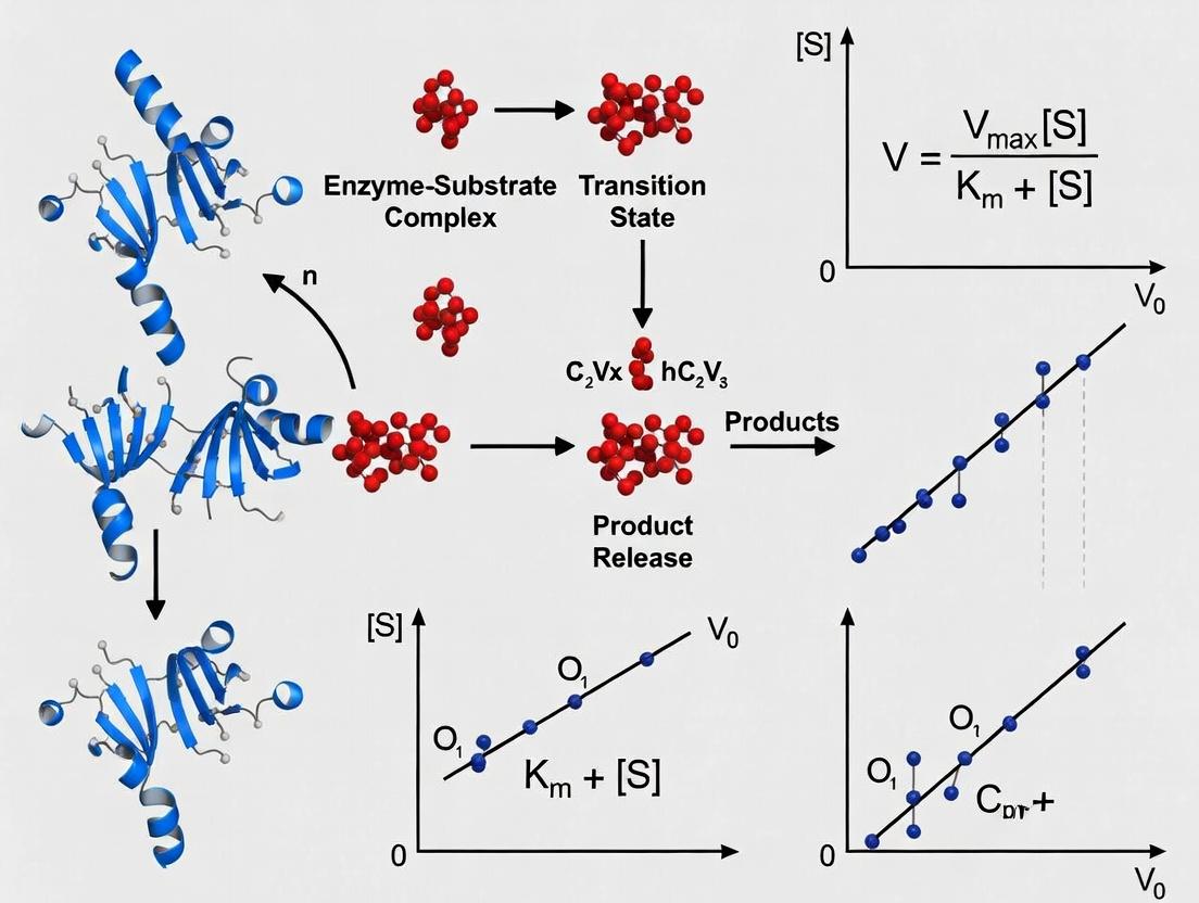
The standard Michaelis-Menten model is derived from a simplified scheme for enzyme-catalyzed reactions, involving the formation of an enzyme-substrate (ES) complex and its subsequent conversion to product.

Diagram 1: Michaelis-Menten enzyme catalysis mechanism.

The derivation applies the steady-state approximation, assuming the concentration of the ES complex remains constant over time. This leads to the classic Michaelis-Menten equation:

v = (Vmax * [S]) / (Km + [S])

Where:

• v is the initial reaction velocity.
• [S] is the substrate concentration.
• Vmax is the maximum reaction velocity, equal to kcat * [Etotal].
• Km is the Michaelis constant, equal to (k₋₁ + k_cat) / k₁.

Km serves multiple interpretative functions: it approximates the dissociation constant of the ES complex (when k_cat is much smaller than k₋₁), reflects enzyme-substrate affinity, and identifies the enzyme's optimal natural substrate from among several possibilities [1]. In metabolic pathways, the enzyme with the largest Km relative to prevailing substrate concentrations is often considered a rate-limiting step [1].

Experimental Determination of Km: Methodologies and Protocols

The direct experimental approach to determining Km involves measuring initial reaction velocities (v) across a wide range of substrate concentrations ([S]) and fitting the data to the Michaelis-Menten equation.

3.1 Standard Kinetic Assay Protocol A generalized workflow for a spectrophotometric assay, a common method for reactions involving absorbance changes, is as follows [4] [1]:

• Reagent Preparation: Prepare a concentrated stock solution of the purified enzyme and serial dilutions of the substrate in an appropriate assay buffer (containing necessary cofactors, at optimal pH and temperature).
• Initial Rate Measurement: For each substrate concentration, initiate the reaction by adding a small, fixed volume of enzyme to the substrate-buffer mixture. The final enzyme concentration in the assay should be significantly lower than the Km to validly apply the steady-state assumption [5].
• Signal Monitoring: Immediately monitor the formation of product or disappearance of substrate over time (e.g., by absorbance, fluorescence) for a short initial period where the relationship is linear.
• Data Calculation: Calculate the initial velocity (v) for each [S] from the slope of the linear change in signal, converted to concentration units using an appropriate extinction coefficient or standard curve [4].
• Curve Fitting: Plot v against [S] and fit the data using non-linear regression to the Michaelis-Menten equation to obtain estimates for Vmax and Km. The Lineweaver-Burk double-reciprocal plot (1/v vs. 1/[S]) is a linear transformation used historically but is prone to error propagation and is no longer recommended for fitting primary data [6].

3.2 Innovative Experimental Method: Isothermal Titration Calorimetry (ITC) Beyond optical methods, techniques like Isothermal Titration Calorimetry (ITC) offer label-free alternatives. A 2025 study demonstrated ITC for determining the specificity constant (Γ) of RUBISCO, which is related to the relative Km values for CO₂ versus O₂ [7].

• Protocol: The method involves titrating a CO₂/NaHCO₃ solution into a reaction cell containing RUBISCO, RuBP (substrate), and a fixed O₂ concentration. The heat flow (ΔrH) is measured for each injection.
• Data Analysis: The total measured enthalpy change varies with the substrate ratio ρ ([CO₂]/[O₂]) because the carboxylation and oxygenation reactions have distinct ΔrH values (-62.3 kJ/mol and -401 kJ/mol, respectively). By modeling ΔrH as a weighted sum of these two reaction enthalpies, where the weighting factor is a function of Γ and ρ, the value of Γ can be extracted through non-linear fitting [7].
• Advantage: This method avoids radioactive isotopes and provides a safe, high-throughput alternative for screening engineered RUBISCO variants [7].

The Critical Challenge: Assessing the Accuracy of Determined Km Values

A pivotal issue in modern kinetics is that a Km value obtained via standard nonlinear regression, while precise (with a small reported standard error, SE), can be substantially inaccurate. This inaccuracy arises primarily from systematic errors in the nominal concentrations of enzyme ([E₀]) and substrate ([S₀]) used in the assay, which are not accounted for in routine fitting procedures [2] [3].

4.1 The Accuracy Confidence Interval for Km (ACI-Km) Recent research has introduced the Accuracy Confidence Interval for Km (ACI-Km) framework to address this gap [2] [3]. This method treats the velocity-substrate relationship analogously to a binding isotherm. It propagates user-estimated uncertainties in [E₀] and [S₀] (e.g., from pipetting tolerances, stock solution calibration, or protein quantification methods) through the fitting process to generate a statistically robust interval that has a high probability of containing the true Km value.

• Workflow: Researchers input their kinetic data ([S] and v) and provide confidence intervals for the accuracy of their stock concentrations. The ACI-Km algorithm then calculates the probability distribution of plausible Km values arising from these concentration uncertainties.
• Output: The result is an accuracy confidence interval (e.g., 95% ACI) that quantifies the impact of systematic concentration errors on Km. A free web application (https://aci.sci.yorku.ca) automates this analysis [2].

Diagram 2: Workflow for accuracy assessment of Km (ACI-Km framework).

4.2 Traditional Precision vs. Modern Accuracy Assessment The following table contrasts the traditional and ACI-Km approaches to Km uncertainty.

Table 1: Comparison of Km Uncertainty Assessment Methods

Aspect	Traditional Nonlinear Regression (Km ± SE)	ACI-Km Framework
What it Quantifies	Precision (Random Error): The reproducibility of the fit to the noisy velocity data.	Accuracy (Systematic Error): The propagation of systematic concentration uncertainties into the Km estimate.
Source of Uncertainty	Random noise in the measured reaction velocity (v) signals.	Systematic inaccuracies in the nominal enzyme ([E₀]) and substrate ([S₀]) concentrations.
Typical Software Output	Yes (Standard Error, SE, or confidence interval).	No. Requires specialized framework (e.g., ACI web app) [2].
Primary Utility	Indicates data quality and fit reliability under the model.	Alerts researchers to when concentration calibration must be improved and provides a reliable Km range for downstream applications [3].

Computational Prediction of Km: The Rise of Deep Learning Models

To circumvent the expense and time of experimental kinetics, significant advances have been made in predicting Km values from sequence and structural data using deep learning (DL).

5.1 Model Architectures and Frameworks Models like UniKP and DLERKm represent the state of the art [8] [6]. These frameworks use multi-modal inputs:

• Enzyme Information: Amino acid sequence, processed by protein language models (e.g., ESM-2, ProtT5).
• Substrate/Product Information: Molecular structures represented as SMILES strings or fingerprints, processed by chemical language models (e.g., RXNFP) or graph neural networks.
• Contextual Data: Environmental factors like pH and temperature can be incorporated (e.g., in EF-UniKP) [8].

The models integrate these features using attention mechanisms and ensemble learners to output predictions for kcat, Km, and kcat/Km [8] [6].

Diagram 3: Deep learning framework for predicting enzyme kinetic parameters.

5.2 Performance and Application These models are trained on databases like BRENDA and SABIO-RK. UniKP demonstrated the ability to distinguish wild-type enzymes from mutants and guide the discovery of high-activity tyrosine ammonia lyase (TAL) variants, with some showing a 3.5-fold higher catalytic efficiency than wild-type [8]. DLERKm, which incorporates product information, reported superior performance over previous models, highlighting the importance of full reaction information for accurate prediction [6].

Table 2: Representative Deep Learning Models for Km Prediction

Model Name	Key Input Features	Architectural Highlights	Reported Performance Note
UniKP [8]	Enzyme sequence, Substrate structure (SMILES), pH, Temp.	Pre-trained language models (ProtT5); Ensemble model (Random Forest/Extreme Trees).	Effectively identified high-activity TAL enzymes; EF-UniKP variant incorporates environmental factors.
DLERKm [6]	Enzyme sequence, Substrate & Product structures.	ESM-2 (enzyme), RXNFP (reaction), molecular fingerprints, channel attention.	Incorporating product information improved prediction metrics (e.g., R²) versus enzyme-substrate only models.
MPEK [6]	Enzyme sequence, Substrate structure, pH, Temp, Organism.	ProtT5 (enzyme), Mole-BERT (molecule), gating network.	Integrates multiple contextual factors for prediction.

Integrated Discussion: From Foundational Model to Robust Parameterization

The journey from the classical Michaelis-Menten equation to reliable Km determination embodies the evolution of biochemical research. The equation's enduring strength is its conceptual clarity and practical utility. However, its effective application hinges on recognizing and addressing two modern realities.

First, experimental accuracy is paramount. The ACI-Km framework provides a crucial diagnostic tool, shifting the focus from purely statistical precision to a comprehensive assessment of accuracy. It alerts researchers when their workflow's concentration uncertainties unacceptably blur the biological signal, guiding investment in better calibration or experimental design [2] [3]. This is essential for making confident decisions in enzyme engineering or drug discovery.

Second, computational prediction is a transformative complement. Deep learning models like UniKP and DLERKm are overcoming historical data scarcity to provide fast, in silico estimates of Km [8] [6]. Their primary value lies in prioritization – screening vast protein sequence spaces or mutant libraries to identify the most promising candidates for wet-lab validation, drastically accelerating the design-build-test cycle in metabolic engineering and synthetic biology.

Therefore, a robust thesis on determining Km must advocate for a triangulated approach: using predictive models to generate intelligent hypotheses, executing carefully controlled kinetic experiments to test them, and applying accuracy assessment frameworks like ACI-Km to validate the reliability of the obtained parameters before they feed into higher-order biological models or industrial decisions.

The Scientist's Toolkit: Essential Reagents and Materials

Table 3: Key Research Reagent Solutions for Michaelis-Menten Kinetics

Item	Function & Specification	Critical Considerations
Purified Enzyme	The catalyst of interest. Must be highly purified to avoid interfering activities and accurately quantify [E₀].	Source (recombinant/native), purity (≥95% by SDS-PAGE), storage buffer, and documented specific activity.
Substrate	The molecule upon which the enzyme acts. A range of high-purity stock solutions is required.	Solubility in assay buffer, stability during assay, absence of inhibitory contaminants.
Assay Buffer	Provides the optimal chemical environment (pH, ionic strength). Includes necessary cofactors (Mg²⁺, NADH, etc.).	pH optimum, buffer capacity, chelating agents if needed, compatibility with detection method.
Detection System	Measures the time-dependent formation of product or disappearance of substrate.	Spectrophotometer/Fluorimeter: Requires a chromophore/fluorophore change [4]. Isothermal Titration Calorimeter (ITC): Measures heat change; label-free [7].
Positive Control	A known enzyme with established Km for a standard substrate.	Validates the entire experimental and analytical workflow.
Inhibitor (for studies)	A molecule that reduces enzymatic activity, used to characterize enzyme mechanism.	Known type (competitive/non-competitive) and potency (Ki) [1].
Software	For non-linear regression and advanced analysis (e.g., ACI-Km).	GraphPad Prism, Origin, or specialized tools like the ACI web application [2] [3].

The Michaelis constant (Kₘ) is a fundamental parameter in enzyme kinetics, quantitatively defined as the substrate concentration at which the reaction velocity is half of the maximum velocity (Vₘₐₓ) [9]. This whitepaper frames the precise determination of Kₘ within the broader thesis of robust and reproducible enzyme characterization. Accurate Kₘ values are not mere academic exercises; they are critical for comparing enzyme variants, screening inhibitors, setting physiologically relevant assay conditions, and informing metabolic flux models in systems biology [3]. However, standard experimental and analytical practices can yield values that are precise (indicated by small standard errors) yet inaccurate, leading to potentially costly errors in drug development and bioprocess engineering [3]. This guide synthesizes the mathematical underpinnings, standard and advanced experimental protocols, and modern analytical frameworks essential for rigorous Kₘ determination.

Mathematical Definition and Derivation

The definition of Kₘ emerges from the Michaelis-Menten model of enzyme kinetics. The model is based on the fundamental reaction scheme where an enzyme (E) binds to its substrate (S) to form a complex (ES), which then yields product (P) and regenerates the free enzyme [10].

Core Assumptions for Derivation: Several steady-state assumptions are required: the concentration of the ES complex remains constant during the measured reaction period; the initial substrate concentration [S] vastly exceeds the total enzyme concentration [E]ₜ; and only the initial velocity (v), measured when product accumulation is negligible, is considered [11].

Derivation to the Michaelis-Menten Equation: The rate of ES complex formation is given by k₁[E][S]. The rate of its breakdown is (k₋₁ + k₂)[ES]. Applying the steady-state assumption (rate of formation = rate of breakdown) gives: k₁[E][S] = (k₋₁ + k₂)[ES]

Since the total enzyme is partitioned between free and bound states ([E]ₜ = [E] + [ES]), [E] can be substituted with ([E]ₜ - [ES]). Solving for [ES] yields: [ES] = ([E]ₜ [S]) / ( (k₋₁+k₂)/k₁ + [S] )

The Michaelis constant Kₘ is defined as the composite rate constant (k₋₁ + k₂)/k₁ [11]. The observed reaction velocity v is proportional to [ES] (v = k₂[ES]), and the maximum velocity Vₘₐₓ occurs when all enzyme is saturated (Vₘₐₓ = k₂[E]ₜ). Substituting these relationships produces the Michaelis-Menten equation: v = (Vₘₐₓ [S]) / (Kₘ + [S]) [10] [12]

Operational Definition of Kₘ: When the reaction velocity v is half of Vₘₐₓ (v = Vₘₐₓ/2), the equation simplifies to: Vₘₐₓ/2 = (Vₘₐₓ [S]) / (Kₘ + [S]) Solving for [S] confirms that Kₘ = [S] when v = Vₘₐₓ/2. Thus, Kₘ is the substrate concentration required for half-maximal enzymatic activity [9]. Graphically, it is the x-axis coordinate of the hyperbolic Michaelis-Menten curve at the half-saturation point.

Diagram 1: Fundamental Enzyme Kinetic Pathway. This scheme shows the reversible formation of the enzyme-substrate complex (ES) and its irreversible catalysis to product, governed by rate constants k₁, k₋₁, and k₂.

Experimental Determination of Kₘ

Standard Initial Rate Method

The classical method involves measuring initial reaction velocities (v) at a minimum of six to eight different substrate concentrations spanning a range from approximately 0.2Kₘ to 5Kₘ [9].

Detailed Protocol:

• Reaction Setup: Prepare a master mix containing buffer, cofactors, and any fixed substrates. Maintain a constant, catalytically relevant temperature (e.g., 25°C or 37°C).
• Substrate Variation: Dispense aliquots of the master mix. Add a different concentration of the target substrate (the one for which Kₘ is being determined) to each reaction vessel. The highest concentration should aim to saturate the enzyme.
• Reaction Initiation: Start all reactions by adding a fixed, low concentration of enzyme. The enzyme must be the final component added to ensure accurate timing.
• Initial Velocity Measurement: Immediately monitor the appearance of product or disappearance of substrate for a short, linear period (typically ≤5% substrate conversion). Use a method appropriate for the reaction (e.g., spectrophotometry for NADH oxidation at 340 nm, fluorometry, or chromatography) [9].
• Data Collection: Record the slope of the linear progress curve for each [S] as the initial velocity (v), expressed in units like µM·s⁻¹.

Optimal Experimental Design: Research indicates that for progress curve analysis (a related method), the most precise estimate of Kₘ is obtained when the initial substrate concentration [S]₀ is chosen to be approximately 2 to 3 times the expected Kₘ value [13].

Data Analysis and Linear Transformations

The hyperbolic v vs. [S] data is fit to the Michaelis-Menten equation using non-linear regression (preferred), often via software like GraphPad Prism or KaleidaGraph [9]. Historically, linear transformations are used for visualization and preliminary estimation.

Lineweaver-Burk Plot: The double-reciprocal plot (1/v vs. 1/[S]) is the most common linear form. The y-intercept is 1/Vₘₐₓ, the x-intercept is -1/Kₘ, and the slope is Kₘ/Vₘₐₓ [14]. It is prone to distortion at low [S]. Eadie-Hofstee Plot: Plotting v vs. v/[S] yields a slope of -Kₘ and a y-intercept of Vₘₐₓ. This method spreads data more evenly but can be sensitive to experimental error. Hanes-Woolf Plot: Plotting [S]/v vs. [S] gives a slope of 1/Vₘₐₓ and an x-intercept of -Kₘ. It offers a better error structure than the Lineweaver-Burk plot.

Table 1: Comparison of Linear Transformations for Michaelis-Menten Analysis

Plot Type	Axes	Slope	Y-Intercept	X-Intercept	Primary Advantage	Primary Disadvantage
Lineweaver-Burk	1/v vs. 1/[S]	Kₘ/Vₘₐₓ	1/Vₘₐₓ	-1/Kₘ	Intuitive, widely used.	Compresses data at high [S]; exaggerates error at low [S].
Eadie-Hofstee	v vs. v/[S]	-Kₘ	Vₘₐₓ	Vₘₐₓ/Kₘ	Errors are not transformed, spreading data evenly.	Both variables depend on v, correlating errors.
Hanes-Woolf	[S]/v vs. [S]	1/Vₘₐₓ	Kₘ/Vₘₐₓ	-Kₘ	Better error distribution than Lineweaver-Burk.	Less intuitive for direct parameter estimation.

Advanced Method: Integrated Rate Equation (Progress Curve) Analysis

Instead of measuring multiple initial rates, this method fits a single progress curve (product vs. time) to the integrated form of the Michaelis-Menten equation. One design proposes using an initial [S]₀ of 2-3Kₘ for optimal Kₘ estimation precision [13]. This method uses all data points from a single reaction but requires accounting for product inhibition and substrate depletion.

Diagram 2: Workflow for Determining Michaelis Constant (Kₘ). The process highlights two primary methodological paths converging on non-linear regression and modern accuracy assessment.

Quantitative Interpretation and Benchmarking

Kₘ values are expressed in molarity (M) and provide a measure of enzyme-substrate affinity. A lower Kₘ indicates higher apparent affinity, as less substrate is needed to achieve half-saturation. It is critical to note that Kₘ is not a direct dissociation constant (Kd) unless k₂ << k₋₁ (the rapid equilibrium assumption). In the standard steady-state derivation, Kₘ = (k₋₁ + k₂)/k₁, so it is always ≥ Kd [11].

Table 2: Representative Kₘ Values for Selected Enzymes and Substrates

Enzyme	Substrate	Approximate Kₘ	Biological/Experimental Implication
Hexokinase IV (Glucokinase)	Glucose	8-10 mM [9]	High Kₘ in liver allows sensing of blood glucose levels over a wide range.
Hexokinase I	Glucose	0.05 mM [9]	Low Kₘ in muscle ensures efficient uptake/utilization even at low glucose.
Lactate Dehydrogenase (Heart, LDH-B)	NADH (with pyruvate saturating)	~5-15 µM (varies by isoform) [9]	Isozyme-specific Kₘ aids in tissue-specific metabolic control.
Carbonic Anhydrase	CO₂	~12 mM	High turnover number (k_cat) compensates for low apparent affinity.
β-Galactosidase	Lactose	~0.8 mM	Reflects physiological concentration of its substrate.
Acetylcholinesterase	Acetylcholine	~0.1 mM	Efficient clearance of neurotransmitter at the synapse.

Practical Implications and Advanced Considerations

Inhibition Kinetics

Kₘ is a key diagnostic parameter in characterizing enzyme inhibitors [9]:

• Competitive Inhibition: Inhibitor competes with substrate for the active site. Apparent Kₘ increases, Vₘₐₓ remains unchanged.
• Non-Competitive Inhibition: Inhibitor binds elsewhere, reducing effective enzyme concentration. Apparent Vₘₐₓ decreases, Kₘ remains unchanged.
• Uncompetitive Inhibition: Inhibitor binds only to the ES complex. Both apparent Vₘₐₓ and Kₘ decrease.

The Critical Challenge of Accuracy vs. Precision

A pivotal 2025 study highlights a major gap in standard practice: traditional non-linear regression reports the precision of Kₘ (standard error, SE) but not its accuracy—the closeness to the true value. Systematic errors in the nominal concentrations of enzyme ([E]₀) and substrate ([S]₀) can lead to Kₘ estimates that are precise but highly inaccurate [3].

Solution: The Accuracy Confidence Interval (ACI) Framework: This modern framework treats Kₘ determination analogously to a binding-isotherm regression. It propagates user-estimated uncertainties in [E]₀ and [S]₀ (e.g., from pipetting, stock solution preparation) to calculate an ACI that is expected to contain the true Kₘ value with a specified confidence level [3]. This is crucial for valid comparisons (e.g., between enzyme mutants) and reliable decision-making in drug discovery. A free web application automates this analysis [3].

The Scientist's Toolkit: Essential Research Reagents

Table 3: Key Reagent Solutions for Kₘ Determination Assays

Reagent/Material	Function in Kₘ Assay	Critical Considerations
Purified Enzyme	The catalyst under study. Its concentration must be known accurately and kept constant across all [S] conditions.	Purity and activity must be validated. Stock concentration error is a major source of inaccuracy in Kₘ [3].
Target Substrate	The reactant whose concentration is varied to determine Kₘ.	High-purity stock with accurately known concentration is essential. Serial dilutions must be prepared precisely.
Cofactors (e.g., NADH, Mg²⁺)	Essential for the catalytic activity of many enzymes.	Must be included at saturating, non-limiting concentrations when not the variable substrate [9].
Reaction Buffer	Maintains optimal and constant pH, ionic strength, and chemical environment.	Buffer composition and pH can significantly affect enzyme kinetics and must be controlled.
Coupled Assay Enzymes (if used)	Used in indirect assays to continuously monitor product formation (e.g., linking ATP production to NADH oxidation).	Must be in excess to ensure the measured rate is limited only by the primary enzyme.
Spectrophotometer/Fluorometer	Instrument for monitoring the reaction progress (e.g., absorbance change of NADH at 340 nm).	Must have stable temperature control and precise timers for initial rate measurements.
Microplate Reader or Cuvettes	Reaction vessels.	Ensure path length is known and consistent for accurate concentration calculations from absorbance.

The rigorous determination of the Michaelis constant (Kₘ) is a cornerstone of quantitative enzymology with profound implications for basic research and applied biotechnology. While its mathematical definition as [S] at half-Vₘₐₓ is elegantly simple, obtaining an accurate and meaningful value demands careful experimental design, appropriate data analysis, and—as underscored by the latest research—an awareness of the distinction between precision and true accuracy [3].

Future research in this field, as part of a comprehensive thesis on Michaelis constant determination, should focus on the widespread adoption of accuracy-assessment frameworks like ACI, the development of standardized reporting guidelines that include uncertainty budgets for [E]₀ and [S]₀, and the integration of these robust kinetic parameters into predictive computational models of cellular metabolism. By moving beyond reporting only a Kₘ value with a standard error to reporting a value with a validated Accuracy Confidence Interval, researchers can ensure their findings are reliable, reproducible, and truly informative for downstream applications in drug development and systems biology.

Within the framework of a broader thesis on determining the Michaelis constant (Km), this guide provides an in-depth technical examination of the two principal theoretical approaches used to derive this fundamental kinetic parameter. The Michaelis constant is a cornerstone of enzymology, quantitatively describing the relationship between an enzyme's catalytic rate and substrate concentration [15]. Its accurate determination is critical for researchers, scientists, and drug development professionals seeking to characterize enzyme mechanisms, understand metabolic pathways, and design effective inhibitors [16] [17].

The canonical Michaelis-Menten equation, v₀ = (Vmax[S])/(Km + [S]), describes a hyperbolic relationship where v₀ is the initial velocity, [S] is the substrate concentration, and Vmax is the maximum velocity [10] [18]. The parameter Km, the substrate concentration at which the reaction velocity is half of Vmax, can be interpreted differently based on the underlying mathematical assumptions used in its derivation [19]. The two classical derivations—the Rapid Equilibrium Approximation and the Steady-State (or Briggs-Haldane) Approximation—rest on different premises about the behavior of the enzyme-substrate complex (ES). These derivations yield identical mathematical forms for the rate equation but assign distinct biochemical meanings to Km [20] [19]. This whitepaper will dissect these methodologies, detail associated experimental protocols, and explore advanced modern approaches for robust Km determination.

Theoretical Foundations and Mathematical Derivations

The basic reaction scheme for a single-substrate, irreversible enzyme-catalyzed reaction is: E + S ⇌ ES → E + P where E is the free enzyme, S is the substrate, ES is the enzyme-substrate complex, and P is the product. The rate constants are defined as k₁ (forward binding), k₋₁ (dissociation of ES), and kcat (or k₂, the catalytic rate constant for product formation) [10] [18].

The Rapid Equilibrium (Michaelis-Menten) Derivation

The rapid equilibrium approximation assumes that the binding step (E + S ⇌ ES) is significantly faster than the catalytic step (ES → E + P). Consequently, the enzyme, substrate, and complex are considered to be in instantaneous equilibrium [20] [18]. The equilibrium dissociation constant for the ES complex, Ks (often synonymous with Kd), is defined as: Ks = [E][S]/[ES] = k₋₁/k₁ By applying the enzyme conservation equation ([E]₀ = [E] + [ES]) and recognizing that the initial velocity v₀ = kcat[ES], algebraic substitution leads to the familiar Michaelis-Menten equation: v₀ = (kcat[E]₀[S]) / (Ks + [S]) In this derivation, the Michaelis constant Km is explicitly equal to the dissociation constant Ks (or Kd). Therefore, Km is a true thermodynamic equilibrium constant, inversely related to the enzyme's affinity for the substrate: a lower Km indicates tighter binding [19] [21].

The Steady-State (Briggs-Haldane) Derivation

The steady-state approximation, formulated by Briggs and Haldane, is a more general condition. It assumes that over the measurable course of the reaction, the concentration of the ES complex remains constant because its rate of formation equals its rate of consumption [22]. This does not require the binding step to be at equilibrium. The steady-state condition is expressed as: d[ES]/dt = 0 = k₁[E][S] – (k₋₁ + kcat)[ES]. Again, using the enzyme conservation law and v₀ = kcat[ES], solving for [ES] yields: v₀ = (kcat[E]₀[S]) / ([(k₋₁ + kcat)/k₁] + [S]) The equation is identical in form to the rapid equilibrium result, but the Michaelis constant is now defined as: Km = (k₋₁ + kcat) / k₁ In this framework, Km is a kinetic parameter, not a pure equilibrium constant. It represents the substrate concentration at which the reaction velocity is half of Vmax, but its relationship to binding affinity (Kd = k₋₁/k₁) is modulated by the catalytic rate kcat [19].

Table 1: Comparative Analysis of Derivation Assumptions and Outcomes

Aspect	Rapid Equilibrium Approximation	Steady-State Approximation
Core Assumption	The enzyme-substrate binding step is at instantaneous equilibrium.	The concentration of the ES complex is constant over time (formation rate = breakdown rate).
Condition	k₋₁ >> kcat. Substrate dissociation is much faster than catalysis.	No specific requirement on the relative magnitudes of k₋₁ and kcat. More general.
Definition of Km	Km = Ks = k₋₁/k₁	Km = (k₋₁ + kcat)/k₁
Relationship to Kd	Km is identical to the dissociation constant Kd.	Km ≥ Kd. They are equal only if kcat << k₋₁.
Physical Meaning	A pure thermodynamic binding constant. Measure of substrate affinity.	A kinetic constant representing [S] at ½Vmax. Governed by both binding and catalysis.
Primary Citation	Michaelis & Menten (1913) [18]	Briggs & Haldane (1925) [22] [17]

Table 2: Quantitative Implications of the Relationship Between Km and Kd

Condition	Mathematical Relationship	Practical Implication for Interpretation
kcat << k₋₁ (Slow Catalysis)	Km ≈ Kd	Km reliably reflects substrate binding affinity. Rapid equilibrium assumption is valid.
kcat ≈ k₋₁	Km > Kd	Km overestimates the true binding affinity (Kd).
kcat >> k₋₁ (Fast Catalysis)	Km >> Kd	Km is a poor indicator of binding affinity. Steady-state assumption is essential.
General Case	Km / Kd = 1 + (kcat/k₋₁)	The ratio quantifies the deviation; Km is always greater than or equal to Kd [19].

Experimental Methodologies for Determining Km

Accurate determination of Km relies on measuring initial reaction velocities (v₀) across a range of substrate concentrations while maintaining a constant, low enzyme concentration to meet the model's assumptions [15] [17].

Initial Velocity (Progress Curve) Assays

The classical method involves measuring the initial linear phase of product formation or substrate depletion for multiple reactions, each with a different initial [S]₀. Detailed Protocol:

• Reaction Mixture: Prepare a master mix containing all non-varying components (buffer, cofactors, salts, enzyme). The buffer must control pH, as it significantly affects enzyme activity and Km [23].
• Initiation: Dispense aliquots of the master mix into vessels containing varying concentrations of substrate. Start the reaction by adding enzyme or substrate, ensuring rapid mixing.
• Continuous Monitoring: Use a spectrophotometer, fluorometer, or other detector to monitor the change in signal (e.g., absorbance of product) over time, typically for the first 5-10% of substrate conversion.
• Initial Rate Calculation: Determine the slope of the linear portion of the progress curve for each [S]₀. This slope is v₀, expressed in concentration/time (e.g., µM/s) [15].
• Data Fitting: Plot v₀ vs. [S]₀ and fit the data to the Michaelis-Menten equation using non-linear regression, which is the preferred and most accurate method. Alternatively, linear transformations like the Lineweaver-Burk plot (1/v vs. 1/[S]) can be used but are sensitive to experimental error [10] [23].

Advanced & Computational Approaches

Modern methods address limitations of the classic assay, such as the requirement for high substrate concentrations or prior knowledge of Km.

• Total Quasi-Steady-State Approximation (tQSSA): For conditions where the standard assumption ([E]₀ << [S]₀ + Km) is violated (e.g., in vivo or high-enzyme conditions), the tQSSA model provides a more robust framework for analyzing full progress curves without being restricted to initial rates [17].
• Approximate Bayesian Computation (ABC): A likelihood-free statistical method that can estimate Km and kcat from a single progress curve, reducing reagent use and time. It is particularly useful when enzyme or substrate is limiting [16].
• Response Surface Methodology (RSM): A statistical technique that models Km and Vmax as functions of multiple interacting environmental variables (e.g., pH, temperature, inhibitor concentration) simultaneously, providing a more comprehensive understanding of enzyme behavior under different conditions [23].

Diagram 1: Workflow for Experimental Determination of Km

The Scientist's Toolkit: Essential Reagents and Materials

Table 3: Key Research Reagent Solutions for Km Determination Assays

Reagent/Material	Function & Purpose	Critical Specifications & Notes
Purified Enzyme	The catalyst under investigation. Source (recombinant, tissue) and purity are critical for reproducible kinetics.	Maintain activity: store in appropriate buffer, often at -80°C with stabilizers (e.g., glycerol, BSA). Aliquot to avoid freeze-thaw cycles.
Substrate	The molecule converted by the enzyme. Must be highly pure and compatible with the detection method.	Solubility at high concentrations can be limiting. Prepare fresh stock solutions to avoid hydrolysis/oxidation. Use kinetic, not thermodynamic, solubility.
Assay Buffer	Maintains constant pH and ionic strength, providing optimal and stable enzyme activity.	Choice of buffer (e.g., Tris, phosphate, HEPES) depends on enzyme and pKa. Include essential cations (Mg²⁺, etc.) and DTT to prevent oxidation.
Detection System	Quantifies the formation of product or depletion of substrate over time.	Spectrophotometric: Requires a chromogenic change (NADH at 340 nm is common). Fluorometric: Higher sensitivity (e.g., fluorogenic substrates). Coupled Assay: Uses a second enzyme to generate a detectable signal [15] [23].
Positive Control	Validates the functionality of the assay system.	A known substrate or an enzyme batch with previously characterized Km.
Inhibitor/Negative Control	Confirms signal specificity.	A reaction lacking enzyme or containing a known specific inhibitor to measure non-enzymatic background.
Microplate Reader / Spectrophotometer	Instrument for high-throughput or cuvette-based kinetic measurements.	Must have precise temperature control (e.g., Peltier) and rapid mixing capabilities. Software for initial rate calculation is essential.
Data Analysis Software	For non-linear regression and statistical analysis of kinetic data.	Tools like GraphPad Prism, SigmaPlot, or dedicated packages for Bayesian (ABC) or tQSSA analysis [16] [17] [23].

Advanced Kinetic Models and Future Directions

The standard Michaelis-Menten model, while foundational, has limitations. Advanced models extend its utility:

• Total Quasi-Steady-State Approximation (tQSSA): As implemented in modern Bayesian approaches, this model remains accurate even when enzyme concentration is not negligible compared to substrate and Km, a common scenario in cellular environments. It allows for the pooling of data from experiments with different enzyme concentrations, leading to more robust parameter estimation [17].
• Single-Molecule Kinetics: Moves beyond ensemble averages to observe the stochastic behavior of individual enzyme molecules, revealing heterogeneities and transient states masked in traditional assays.
• Machine Learning Integration: Emerging techniques use large kinetic datasets to predict Km values or identify novel modulators, accelerating drug discovery and enzyme engineering.

Diagram 2: Evolution of Kinetic Models Beyond Classic Michaelis-Menten

The derivation of Km via the steady-state or rapid equilibrium approximation is not merely a historical or academic distinction; it has profound implications for the interpretation of this ubiquitous parameter. The rapid equilibrium derivation posits Km as a direct measure of substrate binding affinity (Kd). In contrast, the more general steady-state derivation defines Km as a kinetic constant that incorporates both binding (k₁, k₋₁) and catalytic (kcat) efficiency. For the practicing scientist, the choice of experimental design and data analysis model—from classic initial velocity assays to modern tQSSA and Bayesian methods—should be informed by the system's biochemistry and the specific conditions of the experiment. Accurate Km determination remains a vital endeavor, providing indispensable insights for basic enzymology, drug discovery, and understanding the kinetic constraints of biological networks.

The Michaelis constant (Km) is far more than a simple curve-fitting parameter extracted from a hyperbolic plot. It is a fundamental descriptor of enzyme function that sits at the intersection of biochemistry, cellular physiology, and quantitative systems biology [15]. Its accurate interpretation is critical for tasks ranging from designing basic enzyme assays to constructing predictive metabolic models and designing targeted therapeutics [24]. Misinterpretation of Km can lead to flawed biological conclusions or inefficient biotechnological processes. This guide frames the multidimensional interpretation of Km within the broader thesis of rigorous Michaelis constant research, emphasizing that understanding what Km means is inextricably linked to understanding how it is reliably determined and the conditions under which it is measured [2] [24]. For researchers and drug development professionals, a nuanced grasp of Km is essential for selecting enzyme variants, screening inhibitors, and predicting in vivo enzyme behavior from in vitro data [6].

Theoretical Foundations: The Dual Interpretations of Km

The Km value, defined as the substrate concentration at which the reaction velocity is half of Vmax, admits two primary interpretations, each valid under specific mechanistic assumptions [15] [25].

The Operational Definition: A Measure of Apparent Affinity

The most common and robust interpretation is operational. A lower Km value indicates that an enzyme achieves half its maximum velocity at a lower substrate concentration. This is widely described as the enzyme having a higher apparent affinity for its substrate [26] [27]. Conversely, a higher Km suggests lower apparent affinity. This interpretation is always valid when using the Michaelis-Menten equation to describe steady-state kinetics, regardless of the underlying reaction mechanism [28]. It is immensely useful for comparing different enzymes or the same enzyme under different conditions (pH, temperature, presence of inhibitors).

The Mechanistic Definition: Relating to Rate Constants

Under a specific and common mechanistic condition—where the dissociation of the enzyme-substrate complex (ES) back to enzyme and substrate is much faster than the formation of product (i.e., k₋₁ >> k₂)—Km simplifies to k₋₁/k₁ [25] [28]. In this scenario, Km approximates the dissociation constant (Kd) of the ES complex. This equates Km directly with binding affinity: a lower Km reflects a tighter, more stable ES complex. It is crucial to recognize that this is a special case. In the full Michaelis-Menten derivation (Km = (k₋₁ + k₂)/k₁), Km is a function of both binding (k₁, k₋₁) and catalytic (k₂) rate constants. Therefore, while Km often correlates with affinity, it is more accurately a "specificity constant" that reflects an enzyme's efficiency at low substrate concentrations [29].

Table 1: Comparative Summary of Km Interpretations

Interpretation	Definition	Key Assumption	Primary Utility
Operational (Apparent Affinity)	[S] at which v₀ = Vmax/2 [15]	Steady-state conditions	Comparing enzymes & conditions; assay design
Mechanistic (Dissociation Constant)	Km ≈ k₋₁/k₁ [25]	k₋₁ >> k₂ (rapid equilibrium)	Relating kinetics to binding thermodynamics
Efficiency (Specificity Constant)	Inverse related to kcat/Km [29]	Low [S] conditions	Gauging catalytic perfection & in vivo relevance

Km in Research and Applied Contexts

Diagnostic Tool in Enzyme Inhibition Studies

Changes in Km are a primary diagnostic for determining the mechanism of enzyme inhibition, which is fundamental to pharmacology and drug discovery [27].

• Competitive Inhibition: The inhibitor competes with the substrate for the active site. This increases the apparent Km (more substrate is needed to reach half-saturation), while Vmax remains unchanged [26] [27].
• Non-Competitive & Mixed Inhibition: The inhibitor binds at an allosteric site. Vmax is decreased, while Km may remain unchanged (pure non-competitive) or either increase or decrease (mixed) [27].
• Uncompetitive Inhibition: The inhibitor binds only to the ES complex. This paradoxically decreases the apparent Km (stabilizes ES binding) while also decreasing Vmax [27].

Table 2: Effect of Inhibitor Types on Kinetic Parameters

Inhibition Type	Binding Site	Effect on Vmax	Effect on Apparent Km	Diagnostic Clue
Competitive	Active Site	Unchanged	Increases [27]	Reversible by high [S]
Non-Competitive	Allosteric Site	Decreases	Unchanged [27]	Not reversed by high [S]
Uncompetitive	ES Complex	Decreases	Decreases [27]	Rare; common in multi-substrate rxn
Mixed	Allosteric Site	Decreases	Increases or Decreases [27]	Complex kinetics

Physiological Relevance and the Critical Link to In Vivo Conditions

A Km value's most significant biological meaning lies in its relationship to physiological substrate concentrations [24]. An enzyme's Km relative to the in vivo concentration of its substrate ([S]_physio) dictates its operational point on the activity curve and its sensitivity to substrate fluctuations.

• If [S]_physio << Km: The enzyme operates in the first-order range, where velocity is highly sensitive to changes in substrate concentration. This is typical for regulated enzymes controlling metabolic flux.
• If [S]_physio ≈ Km: The enzyme operates at half its capacity, allowing for potent regulation by factors that modestly alter Km or [S].
• If [S]_physio >> Km: The enzyme is nearly saturated and operates at near-maximal velocity (zero-order kinetics), buffering its activity against substrate changes.

Therefore, interpreting a Km value in isolation is of limited use. Its true physiological meaning emerges from comparison with actual cellular substrate levels. This underscores a major challenge in enzyme kinetics: many reported Km values are derived from assays under non-physiological conditions of pH, temperature, buffer, and ionic strength, which can alter Km significantly and limit their biological predictive power [24].

Methodological Framework: Determining Accurate and Meaningful Km Values

Core Experimental Protocol for Reliable Km Determination

The following detailed protocol is based on standard steady-state kinetics and highlights critical steps for generating reliable data.

1. Initial Rate Assay Establishment:

• Principle: Km and Vmax are defined using initial velocities (v₀), measured when [S] >> [E] and product accumulation is minimal (<5% of [S]), ensuring [S] is constant and reverse reactions/product inhibition are negligible [24] [28].
• Procedure: For each substrate concentration, prepare a reaction mixture with all components except the initiating reagent (e.g., enzyme or cofactor). Pre-incubate at the assay temperature. Initiate the reaction and monitor product formation or substrate depletion continuously (via spectrophotometry, fluorometry) or at multiple early time points. Plot signal vs. time; the linear slope is v₀.

2. Substrate Concentration Range Selection:

• Use a minimum of 8-10 different substrate concentrations, spaced appropriately to define the hyperbolic curve. The range should ideally span 0.2-5.0 times the estimated Km to capture both the first-order and zero-order regions [15].

3. Data Analysis and Curve Fitting:

• Plot v₀ versus [S]. Fit the data directly to the Michaelis-Menten equation (v₀ = (Vmax*[S])/(Km + [S])) using non-linear regression [2].
• Critical Consideration: While the Lineweaver-Burk double-reciprocal plot (1/v vs. 1/[S]) linearizes the data, it disproportionately weights data points at low [S], which often have the highest error. It should be used for visualization and inhibitor diagnosis, not as the primary fitting method [15].

4. Accuracy Assessment (ACI-Km Framework):

• Recent advancements stress that a small standard error (SE) from regression does not guarantee accuracy. Systematic errors in enzyme or substrate concentration ([E]₀, [S]₀) propagate into Km [2].
• Apply the Accuracy Confidence Interval for Km (ACI-Km) [2]. This method uses estimated intervals for [E]₀ and [S]₀ accuracy (from calibration, reagent specs) to calculate a probabilistic interval for Km, providing a more reliable bound for decision-making. A free web application (https://aci.sci.yorku.ca) implements this.

Advanced & Emerging Methodologies

• Isothermal Titration Calorimetry (ITC): Directly measures binding affinity (Kd) and thermodynamics, providing a complementary view to kinetic Km.
• Computational Prediction (Deep Learning): Models like DLERKm now predict Km values from enzyme sequence and substrate/product structures, useful for high-throughput screening and metabolic engineering [6]. These models use pre-trained language models (e.g., ESM-2 for proteins) and reaction fingerprints as inputs.

Table 3: Overview of Computational Km Prediction Methods

Model Name	Core Architecture	Key Input Features	Reported Advantage
DLERKm [6]	ESM-2, RXNFP, Attention	Enzyme seq, Substrate, Product	Incorporates product info for first time
UniKP [6]	ProtT5, SMILES Transformer	Enzyme seq, Substrate	Ensemble model for robustness
MPEK [6]	ProtT5, Mole-BERT	Enzyme seq, Substrate, pH, Temp	Includes environmental factors

Table 4: Key Research Reagent Solutions for Km Determination

Reagent/Material	Function & Importance	Considerations for Accuracy
High-Purity Enzyme	The catalyst of interest. Source (recombinant, purified native) and purity affect specific activity and stability.	Accurate quantification of active site concentration ([E]₀) is critical but challenging. Use activity titrations where possible [2].
Characterized Substrate	The molecule whose transformation is studied. Purity and stability are paramount.	Accurate preparation of stock concentrations ([S]₀) is a major source of systematic error. Use certified standards and precise gravimetry [2].
Physiomimetic Assay Buffer	Maintains pH, ionic strength, and provides necessary cofactors.	Buffer composition (e.g., phosphate vs. Tris) can activate or inhibit enzymes [24]. Strive for physiological relevance (pH, ions, temperature).
Detection System	Measures product formation/substrate depletion (e.g., spectrophotometer, fluorometer, HPLC).	Must have sufficient sensitivity and a linear range suitable for measuring low initial velocities.
Reference Databases	Sources for literature values and metadata (e.g., BRENDA, SABIO-RK, STRENDA) [24].	Essential for comparison. STRENDA guidelines promote reporting standards for reproducibility [24]. Always note EC number and organism [29].

Interpreting Km requires a multidimensional perspective that integrates its operational definition as an apparent affinity constant, its mechanistic relationship to rate constants, and, most importantly, its physiological context relative to in vivo substrate concentrations. Robust Km determination hinges on meticulous initial-rate experiments, awareness of systematic errors in concentration measurements, and the application of modern accuracy assessment frameworks like ACI-Km [2].

Future research in this field will increasingly bridge high-accuracy experimental determination with computational prediction and machine learning models [6]. The ultimate goal is to generate Km values that are not just precise numbers from an in vitro assay, but accurate parameters that can reliably predict enzyme behavior in the complex, crowded, and regulated environment of the living cell, thereby accelerating rational drug design and metabolic engineering.

Key Assumptions of the Model and Their Experimental Implications

The determination of the Michaelis constant (K_m) is a cornerstone of quantitative enzymology, providing critical insights into enzyme-substrate affinity and catalytic efficiency. This parameter, defined as the substrate concentration at which the reaction velocity is half of its maximum (V_max), is not a direct physical measurement but an estimated constant derived from a kinetic model [18] [9]. The foundational model for this estimation is described by the Michaelis-Menten equation, v = (V_max[S])/(K_m + [S]), which relates the initial velocity (v) of an enzyme-catalyzed reaction to the substrate concentration ([S]) [18] [30].

The practical and accurate determination of K_m is entirely contingent upon experimental conditions that satisfy the key assumptions underpinning this model. Violations of these assumptions lead to systematic errors, misestimation of kinetic parameters, and flawed conclusions about enzyme mechanism or inhibitor potency [31] [32]. Therefore, a rigorous understanding of these assumptions—their theoretical basis, their practical limitations, and the experimental protocols designed to uphold them—is essential for any researcher engaged in characterizing enzymes, designing drugs, or interpreting kinetic data. This guide details these core assumptions, their modern interpretations, and the consequent experimental imperatives for valid K_m determination.

The Core Assumptions: Derivation and Modern Interpretation

The canonical Michaelis-Menten model for a single-substrate, irreversible reaction is represented by the mechanism: E + S ⇌ ES → E + P, where k₁ and k_-1 are the rate constants for complex formation and dissociation, and k_cat (or k₂) is the catalytic rate constant [18] [10].

Table 1: Foundational Assumptions of the Michaelis-Menten Model

Assumption	Mathematical Statement	Theoretical Implication	Historical vs. Modern View
1. Initial Velocity (v₀)	Measurement at t≈0, [P]≈0	Negligible product inhibition or reverse reaction [30].	Originally used to circumvent product inhibition [33]; remains absolute.
2. Steady-State (Briggs-Haldane)	d[ES]/dt = 0	[ES] remains constant over measurement period [30].	More general than rapid equilibrium; widely applied [18].
3. Free Ligand Approximation	[S]₀ ≈ [S]₀total	Total substrate far exceeds bound substrate ([S]₀ >> [E]₀).	Common but not strictly necessary for equation form [32].
4. Single Catalytic Pathway	One ES complex forms one product	Model excludes multiple intermediates or substrates.	Simplification; deviations require more complex models.

The derivation of the rate equation employs the steady-state assumption for the enzyme-substrate complex (ES) [30]. Contrary to common teaching, recent analysis clarifies that the valid application of the Michaelis-Menten equation for parameter estimation requires not just the steady-state condition, but the more specific reactant stationary assumption (RSA). The RSA posits that during the initial transient phase where [ES] builds up, the substrate concentration remains approximately constant and equal to its initial value [S]₀ [32]. This is distinct from and a prerequisite for the steady-state condition in practical experiments.

A critical modern refinement concerns the relationship between enzyme concentration ([E]₀) and K_m. Traditional teaching emphasizes [S]₀ >> [E]₀. However, computational and theoretical work defines a more precise validity boundary: the Michaelis-Menten equation yields accurate estimates of K_m and V_max only when [E]₀ is ≤ 0.01 K_m [31]. At higher enzyme concentrations (0.01K_m < [E]₀ < K_m), the system still follows a hyperbolic relationship, but with a different equation, and estimates from the standard plot become inaccurate [31].

Diagram: The Michaelis-Menten Reaction Mechanism. The central, reversible formation of the ES complex is key to the model's assumptions.

Experimental Implications & Validity Criteria

The theoretical assumptions impose strict, testable criteria on experimental design. Failure to meet these criteria is a major source of error in reported kinetic parameters.

Table 2: Experimental Implications of Model Assumptions

Assumption	Experimental Implication	Consequence of Violation
Initial Velocity (v₀)	Measure velocity at earliest possible time (typically <5% substrate conversion). Use continuous or rapid-quench methods.	Product inhibition, curvature in progress curves, underestimation of true Vmax and inaccurate Km [33].
Reactant Stationary (RSA)	Ensure measurement period is short relative to ES complex buildup time. This often implicitly requires [S]₀ >> [E]₀.	The derived hyperbolic equation does not accurately describe v₀ vs. [S]₀ data, leading to biased parameter fits [32].
[E]₀ ≤ 0.01Km	Use enzyme concentration sufficiently low relative to the unknown Km. May require iterative pilot experiments.	Significant systematic error in estimated Km and Vmax. The error increases as [E]₀/Km ratio increases [31].
Constant [E]₀	Enzyme must be stable and fully active throughout assay. Include stability controls.	Apparent activity loss over time, leading to non-linear progress curves and underestimation of rate.
No Inhibitors/Activators	Purify substrate, use high-purity buffers, account for solvent effects.	Altered apparent Km and Vmax, potentially misinterpreted as allosterism or alternate mechanism.

The most quantitatively defined criterion is the [E]₀ to K_m ratio. Research demonstrates that to keep the estimation error for K_m and V_max below ~10% using standard initial rate experiments, the total enzyme concentration must be ≤ 1% of the K_m value [31]. This is a more stringent condition than often applied in practice. For an enzyme with a K_m of 10 µM, [E]₀ should be 100 nM or lower. This constraint can conflict with the need for a detectable signal, necessitating sensitive detection methods.

Diagram: Workflow for Valid Km Determination. The iterative check on enzyme concentration is critical for parameter accuracy.

Detailed Experimental Protocols for Km Determination

Standard Initial Velocity Method

This is the most common method, directly applying the model's assumptions [9].

Protocol:

• Reagent Preparation: Prepare a master mix containing buffer, cofactors, and any essential salts. Prepare a dilution series of substrate (typically 6-8 concentrations spanning 0.2K_m to 5K_m). Prepare enzyme stock at a concentration such that the final [E]₀ in the assay is ≤ 0.01 × the suspected K_m [31].
• Assay Initiation: Aliquot substrate solutions into cuvettes or microplate wells. Add master mix. Initiate reactions by adding a small volume of enzyme stock with rapid mixing.
• Initial Rate Measurement: Immediately begin monitoring product formation (e.g., via absorbance, fluorescence, luminescence) for a short period (typically 30-120 seconds). Ensure ≤ 5% of substrate is consumed during this period to maintain the initial velocity condition [33].
• Data Analysis: Plot initial velocity (v₀) against substrate concentration ([S]₀). Fit the data directly to the hyperbolic Michaelis-Menten equation (v₀ = (V_max[S]₀)/(K_m + [S]₀)) using non-linear regression software. Avoid using linearized plots (e.g., Lineweaver-Burk) for primary analysis, as they distort error structure [33].

Fixed-Point (Time-Point) Method

This method is useful when continuous monitoring is impractical or when substrate depletion is problematic for initial rate measurement [34].

Protocol:

• Reagent Preparation: As in Section 4.1.
• Reaction Incubation: Initiate multiple, identical reactions at different [S]₀. Instead of monitoring continuously, stop each reaction at a fixed, precise time (t) after initiation (e.g., via acid quench, heat denaturation, or inhibitor).
• Product Quantification: Measure the total amount of product [P] formed in each quenched reaction.
• Data Transformation & Analysis: The measured [P] is related to initial velocity by v₀ ≈ [P]/t, provided t is short. However, a more robust approach is to use the equation: t = (K_m/V_max) * ln([S]₀/([S]₀-[P])) + [P]/V_max. By measuring [P] at a fixed t for various [S]₀, K_m and V_max can be estimated by fitting to this integrated form, which accounts for substrate depletion [34] [33].

Protocol for Validating the [E]₀ Criterion

Given the critical importance of the [E]₀ ≤ 0.01K_m rule [31], the following validation step is recommended.

Protocol:

• Perform an initial parameter estimate using the standard method (Section 4.1) with the lowest feasible [E]₀.
• Using the estimated K_m(est), calculate 0.01 * K_m(est).
• If your assay [E]₀ was greater than this value, repeat the experiment with a lower enzyme concentration. If signal-to-noise becomes too low, a more sensitive detection method is required.
• Confirm that the final estimated K_m is stable and does not systematically shift when [E]₀ is further reduced.

Table 3: Common Methods for Estimating Km and Vmax

Method	Procedure	Primary Data Plot	Advantages	Disadvantages & Assumption Checks
Non-Linear Regression (Direct)	Fit v₀ vs. [S]₀ to hyperbolic function.	v₀ vs. [S]₀ (Hyperbolic)	Most accurate; proper error weighting.	Requires good initial parameter guesses. Must verify [E]₀ ≤ 0.01Km [31].
Lineweaver-Burk (1/v vs. 1/[S])	Linear transformation of MM equation.	Double-reciprocal plot (Linear)	Easy visualization; reveals inhibition type.	Poor statistical practice: compresses low [S] data, magnifies error. Use for visualization only [33].
Eadie-Hofstee (v vs. v/[S])	Alternative linear transformation.	v vs. v/[S] (Linear)	Error distribution better than L-B.	Still less reliable than direct fit. Sensitive to experimental scatter.
Integrated Rate Equation Fit	Fit full time-course data for single [S]₀ or fit [P] at fixed t for multiple [S]₀.	[P] vs. time (Progress Curve)	Uses all data points; accounts for depletion.	Computationally complex; assumes no product inhibition or enzyme instability [33].

The Scientist's Toolkit: Essential Reagents & Materials

Table 4: Key Research Reagent Solutions for Michaelis Constant Determination

Reagent/Material	Function & Purpose	Critical Considerations for Valid Assumptions
Highly Purified Enzyme	The catalyst of interest. Concentration must be known (active concentration is ideal).	Stability is key. Must remain fully active during assay to satisfy constant [E]₀ assumption. Use fresh aliquots and activity controls.
Substrate Stock Solutions	The reactant. Prepared at high concentration for dilution series.	Purity is essential to avoid inhibitors. Concentration must be accurately determined. Solubility must allow for [S]₀ >> [E]₀ condition.
Appropriate Assay Buffer	Maintains constant pH, ionic strength, and provides necessary cofactors (Mg²⁺, etc.).	Must not contain inhibitors. Must optimize pH for activity. Buffering capacity must be high enough to withstand reaction byproducts.
Detection System Reagents	Enables quantification of product formation or substrate depletion (e.g., NADH, chromogenic/fluorogenic probes, coupling enzymes).	Must be in excess to not be rate-limiting. Coupling enzymes must have high activity to avoid lag phases, violating initial rate condition.
Positive Control Inhibitor (Optional)	A known inhibitor (e.g., a transition-state analog) for assay validation.	Verifies that measured activity is specific to the enzyme's active site. Useful for troubleshooting.
Sensitive Detection Instrument	Spectrophotometer, fluorometer, or luminescence plate reader capable of rapid, precise measurement.	Sensitivity is paramount to allow work at very low [E]₀ (≤ 0.01Km) [31]. Rapid sampling is needed for true initial rate.

The process of determining the Michaelis constant is not a simple curve-fitting exercise but a rigorous test of whether an enzyme's behavior conforms to a fundamental physical model under specified conditions. The key assumptions—particularly the reactant stationary assumption and the stringent limit on enzyme concentration relative to K_m—are not mere historical footnotes but active constraints that dictate modern experimental design [31] [32].

For researchers in drug discovery, violating these constraints can lead to mischaracterizing inhibitor mechanisms (e.g., misclassifying competitive vs. non-competitive) or incorrectly calculating inhibitor potency (K_i). For enzymologists, accurate K_m and k_cat values are essential for understanding evolutionary optimization, as the specificity constant (k_cat/K_m) is the fundamental measure of catalytic efficiency [18].

Therefore, robust K_m determination requires: 1) A priori planning to ensure ultra-low enzyme concentrations, 2) Validation that progress curves are linear at all substrate concentrations, and 3) Analysis using direct nonlinear fitting of the hyperbolic equation. Adherence to these principles, rooted in the model's core assumptions, ensures that the extracted Michaelis constant is a true reflection of enzyme biochemistry rather than an artifact of flawed kinetics.

Km Determination in Practice: From Classic Plots to Modern Nonlinear Regression

The determination of the Michaelis constant (K_m) is a cornerstone of quantitative enzymology, providing critical insights into enzyme-substrate affinity, catalytic mechanism, and cellular metabolic regulation [35]. Within the broader context of thesis research focused on K_m determination, the accurate measurement of the initial reaction velocity (v) and the strategic planning of the substrate concentration range ([S]) are not merely preliminary steps but the foundational pillars upon which reliable kinetic parameters are built. This guide provides an in-depth technical framework for designing these core experiments, emphasizing principles essential for researchers, scientists, and drug development professionals aiming to characterize enzymes, identify inhibitors, or engineer biocatalysts [36] [37].

The widely accepted Michaelis-Menten model describes the hyperbolic relationship between v and [S], defined by the equation v = (V_max [S]) / (K_m + [S]), where V_max is the maximum velocity [10] [35]. The K_m value, defined as the substrate concentration at which the reaction velocity is half of V_max, is a key parameter for comparing enzymes from different sources and understanding their physiological context [36]. For competitive inhibitor screening—a primary goal in drug discovery—assays must be conducted with substrate concentrations at or below the K_m to ensure sensitivity to inhibition [36]. Consequently, a well-founded experimental design to measure v and establish a valid [S] range is indispensable for generating robust, publication-quality kinetic data that can inform downstream applications in biotechnology and therapeutics.

Theoretical Foundations: Defining Initial Velocity and Its Imperative

The Concept and Critical Importance of Initial Velocity

The initial velocity (v) of an enzyme-catalyzed reaction is defined as the rate measured during the very early phase of the reaction, specifically when less than 10% of the substrate has been converted to product [36]. Under these conditions, several critical assumptions of the Michaelis-Menten model hold true: the substrate concentration ([S]) remains essentially constant, the accumulation of product (and thus any potential product inhibition or contribution of the reverse reaction) is negligible, and the enzyme-substrate complex [ES] is in a steady state [36] [35].

Adherence to initial velocity conditions is non-negotiable for valid steady-state kinetic analysis. Failure to do so leads to significant artifacts and erroneous parameter estimation [36]:

• Non-linearity with Enzyme Concentration: The reaction rate ceases to be directly proportional to the amount of active enzyme present.
• Uncertain Actual Substrate Concentration: The depletion of substrate makes the starting [S] an inaccurate representation of the conditions during measurement.
• Invalid Kinetic Treatment: The fundamental mathematical derivations of the Michaelis-Menten equation break down, rendering fitted K_m and V_max values unreliable.

The Integrated Rate Equation: An Alternative Approach

While the measurement of initial velocities from the linear portion of progress curves is the classical and most common method, a robust alternative exists. The integrated form of the Michaelis-Menten equation (Eq. 2: t = [P]/V_max + (K_m/V_max) · ln([S]₀/([S]₀ - [P]))) allows for the determination of K_m and V_max by analyzing the complete time course of a single reaction, even when a substantial fraction (theoretically up to 70%) of the substrate is consumed [38]. This method is particularly advantageous when experimental constraints make frequent early time-point sampling difficult, such as with discontinuous assays using HPLC or electrophoretic methods [38]. It is crucial to verify that the enzyme remains stable and that no inhibition (by product or excess substrate) occurs during the extended reaction time when using this approach [38].

Experimental Design and Protocols

Establishing Initial Velocity Conditions: The Reaction Progress Curve Experiment

The first practical experiment in any kinetic characterization is to define the time window over which initial velocity conditions are met for a specific enzyme under specific assay conditions.

Detailed Protocol:

• Prepare Reaction Mixtures: Set up a series of reactions with a fixed, saturating substrate concentration (e.g., [S] > 5 K_m, if a literature value exists) and at least three different enzyme concentrations (e.g., a 2-fold serial dilution series) [36].
• Initiate and Monitor Reaction: Start the reaction by adding enzyme and immediately begin continuous monitoring of product formation or substrate depletion (e.g., via spectrophotometry, fluorimetry).
• Generate Progress Curves: Record the signal over time until the reaction clearly reaches a plateau (substrate exhaustion).
• Analyze for Linearity: Plot the concentration of product (or change in signal) versus time for each enzyme concentration. Identify the early time segment where the progress curve is linear for all enzyme concentrations tested.
• Define the Valid Time Window: The initial velocity (v) for subsequent experiments is the slope of this linear region. The duration of this linear phase dictates the maximum allowable reaction time for all future assays [36]. As shown in foundational texts, reducing the enzyme concentration can extend the period of linearity by slowing substrate depletion [36].

Table 1: Key Design Parameters for Initial Velocity Determination

Parameter	Recommended Design	Rationale & Consequences
Substrate Conversion	< 10% [36]	Maintains constant [S]; prevents product inhibition; validates steady-state assumption.
Enzyme Concentration	Varied (e.g., 3-4 levels) [36]	Identifies a linear time window common to all [E]; ensures v is proportional to [E].
Reaction Time Course	Continuous monitoring preferred [39]	Allows accurate identification of the linear phase; detects lag/burst phases or instability.
Control for Background	Include "no enzyme" and/or "no substrate" controls [36]	Corrects for non-enzymatic substrate decay or signal background.

Planning the Substrate Concentration Range forKmDetermination

Once the linear time window is established, the next step is to design the substrate matrix to generate a saturation curve for fitting K_m and V_max.

Detailed Protocol:

• Determine the Approximate Range: Ideally, use a literature-reported K_m as a guide. In its absence, run a preliminary experiment with 6 substrate concentrations spanning a broad range (e.g., 0.1 µM to 1000 µM) to get an initial estimate [36].
• Design the Final Concentration Series: Based on the preliminary estimate, prepare a minimum of 8 substrate concentrations spaced unevenly to provide more data points near the K_m. The range should typically bracket the K_m, from 0.2 × K_m to 5.0 × K_m [36]. For a more optimized design that minimizes error in the K_m estimate, research suggests using an initial substrate concentration of approximately 2 to 3 times the K_m value when employing integrated progress curve analysis [40].
• Run the Saturation Experiment: For each [S], run the reaction in triplicate within the pre-determined linear time window. Measure the initial velocity (v).
• Ensure Excess Substrate: The total enzyme concentration [E]₀ must be significantly less than the lowest [S] tested (typically [S]/[E] > 100) to satisfy the steady-state assumption [36].

Table 2: Substrate Concentration Range Design for Kinetic Analysis

Analysis Goal	Recommended [S] Range	Key Considerations
Initial Km/Vmax Estimate	6 concentrations, broad log-scale (e.g., 0.1-100 µM) [36]	Captures the full transition from first-order to zero-order kinetics.
Accurate Km/Vmax Fit	8+ concentrations from ~0.2Km to ~5Km [36]	Provides high-density data in the most sensitive part of the hyperbola.
Competitive Inhibitor Screening	[S] ≤ Km (typically [S] = Km) [36]	Maximizes assay sensitivity to inhibitor competition; using [S] >> Km masks inhibitor potency.
Progress Curve Analysis	Initial [S]₀ ≈ 2-3 Km [40]	An experimentally efficient design for extracting parameters from a single time course.

The Critical Role of Enzyme Concentration

A frequently overlooked but critical factor is the absolute concentration of enzyme used. The classic Michaelis-Menten equation assumes [E]₀ << [S]₀ and [E]₀ << K_m. Recent rigorous analysis provides a quantitative boundary: for initial rate experiments to yield accurate K_m and V_max through the standard Michaelis-Menten equation, the enzyme concentration should be ≤ 1% of the K_m value (i.e., [E]₀ ≤ 0.01 K_m) [31]. At higher enzyme concentrations (0.01 K_m < [E]₀ < K_m), the kinetics deviate and require a more complex equation for description [31]. This constraint is essential for planning experiments, especially with high-activity enzymes or when using precious substrates at concentrations near their K_m.

Validating the Assay: Controls and Best Practices

A robust experimental design includes validation steps:

• Linearity of Detection: Before kinetic experiments, establish that the detection system (e.g., spectrophotometer) responds linearly to product concentration across the expected range [36].
• Enzyme Stability (Selwyn's Test): Verify that the product plateau level in progress curves is proportional to the enzyme concentration. Non-proportionality indicates enzyme instability during the assay [36] [38].
• Positive Control Inhibitor: For inhibitor screening assays, include a well-characterized competitive inhibitor to confirm the assay yields the expected potency (IC₅₀ or Kᵢ).

Data Analysis and Interpretation

Fitting Kinetic Data

The preferred method for determining K_m and V_max is non-linear regression of the untransformed data (v vs. [S]) to the Michaelis-Menten equation [35]. While linear transformations like Lineweaver-Burk plots are historically noted, they distort error distribution and are less reliable for parameter estimation. Modern software (e.g., GraphPad Prism, SigmaPlot) performs this non-linear fitting efficiently, providing estimates with standard errors.

Troubleshooting Common Issues

• Poor Fit to Hyperbola: May indicate substrate inhibition at high [S], cooperativity, or the presence of an isozyme mixture.
• Abnormally High K_m: Could suggest suboptimal assay conditions (pH, missing cofactor/activator) or that a surrogate, rather than the natural, substrate is being used [36].
• Irreproducible K_m: Check enzyme purity and stability, and ensure lot-to-lot consistency of all reagents [36].

Advanced and Computational Approaches

The experimental determination of K_m can be resource-intensive. The field is now augmented by computational prediction tools powered by deep learning. These models use enzyme sequence and substrate structure (often encoded as SMILES strings) to predict kinetic parameters [6] [37]. Frameworks like UniKP employ pre-trained language models for proteins (e.g., ProtT5) and substrates to create feature vectors, which are then processed by ensemble machine learning models (e.g., extra trees) to predict K_m, k_cat, and k_cat/K_m with significant accuracy [37]. More recent models like DLERKm further incorporate product information into the feature set, improving prediction performance by better representing the complete enzymatic reaction [6]. These tools are valuable for hypothesis generation, guiding experimental design, and prioritizing enzyme targets or variants for experimental characterization.

The Scientist's Toolkit: Essential Research Reagents and Materials

Table 3: Key Research Reagent Solutions for Kinetic Assays

Reagent / Material	Function & Specification	Critical Notes for Experimental Design
Purified Enzyme Target	Biological catalyst of known sequence, purity, and specific activity [36].	Determine stability under assay conditions. Use consistent lots; confirm absence of contaminating activities.
Native or Surrogate Substrate	Molecule transformed by the enzyme. Mimics natural substrate for assay feasibility [36].	Chemical purity is essential. Ensure an adequate, sustainable supply for full project scope.
Assay Buffer System	Maintains optimal pH, ionic strength, and chemical environment for enzyme activity [36].	Include necessary cofactors (e.g., Mg²⁺ for kinases, NADPH for reductases). Avoid components that inhibit or chelate.
Detection System Components	Enables quantification of reaction progress (e.g., NADH, chromogenic/fluorogenic probes, coupled enzymes) [39].	Must be linear over the expected product range. Coupling enzymes must be in excess and not rate-limiting.
Reference Inhibitor	Known potent inhibitor of the target enzyme (e.g., EDTA for metalloproteases).	Serves as a positive control for assay validation and as a benchmark for screening campaigns.
Inactive Enzyme Mutant	Catalytically dead mutant purified identically to wild-type [36].	Critical control for distinguishing specific enzymatic signal from non-specific background in complex systems.

A meticulous and theoretically sound approach to measuring initial velocity and designing the substrate concentration matrix is fundamental to successful K_m research. This involves first rigorously establishing the linear time window via progress curve analysis, then carefully selecting a substrate range that accurately defines the saturation hyperbola, all while respecting the critical constraint of using a sufficiently low enzyme concentration. Adherence to these principles ensures the collection of high-quality kinetic data. This robust experimental foundation, now potentially augmented by predictive computational models, enables accurate enzyme characterization, reliable drug discovery efforts, and meaningful contributions to the field of enzymology.

The determination of the Michaelis constant (K_m) and the maximum reaction velocity (V_max) constitutes a fundamental objective in enzyme kinetics, with direct implications for drug development, diagnostic enzymology, and understanding metabolic pathways. The K_m, defined as the substrate concentration at half-maximal velocity, provides a quantitative measure of an enzyme's affinity for its substrate and is intrinsic to its biological function [41]. Historically, the direct non-linear fitting of data to the hyperbolic Michaelis-Menten equation was computationally challenging. This led to the development of linear transformation methods, the most famous being the Lineweaver-Burk plot (or double reciprocal plot), introduced by Hans Lineweaver and Dean Burk in 1934 [42].

This whitepaper provides an in-depth technical analysis of the Lineweaver-Burk linearization method. Framed within the broader thesis of K_m determination research, it details the method's derivation and protocol, its application in characterizing enzyme inhibition—a critical aspect of drug discovery—and its severe, often overlooked, statistical limitations. While the plot remains a valuable qualitative teaching and diagnostic tool, contemporary research unequivocally demonstrates that non-linear regression methods are superior for the accurate and precise estimation of kinetic parameters [41] [43] [44].

Theoretical Foundation and Linearization

Mathematical Derivation

The process transforms the non-linear Michaelis-Menten relationship into a linear form. The derivation begins with the standard equation:

( v = \frac{V{max} [S]}{Km + [S]} )

Taking the reciprocal of both sides yields:

( \frac{1}{v} = \frac{Km + [S]}{V{max}[S]} )

This expression can be separated into two terms:

( \frac{1}{v} = \frac{Km}{V{max}[S]} + \frac{[S]}{V_{max}[S]} )

Simplifying results in the Lineweaver-Burk Equation:

( \frac{1}{v} = \left( \frac{Km}{V{max}} \right) \frac{1}{[S]} + \frac{1}{V_{max}} ) [42] [45]

This equation has the linear form y = mx + c, where:

• y = 1/v
• x = 1/[S]
• Slope (m) = K_m / V_max
• y-intercept (c) = 1/V_max
• x-intercept (when y=0) = -1/K_m [46] [45]

The following diagram illustrates this mathematical transformation from the hyperbolic Michaelis-Menten plot to the linear Lineweaver-Burk plot.

Visual Interpretation of the Plot

In the resulting double-reciprocal plot, increasing substrate concentration corresponds to moving leftward along the x-axis (as 1/[S] decreases). A higher reaction velocity corresponds to moving downward on the y-axis (as 1/v decreases). The plot is often extended into the negative x-intercept region, which is a mathematical extrapolation without physical reality for substrate concentration but is critical for graphically determining K_m* [46].

Experimental Protocol and Data Analysis

Step-by-Step Methodology

The following protocol is adapted from established enzymology practices and software guides for kinetic analysis [47].

• Reaction Rate Assay: For a fixed enzyme concentration, measure the initial velocity (v) of the reaction at multiple, carefully chosen substrate concentrations ([S]). It is crucial to ensure measurements are taken during the initial linear phase of product formation.
• Data Transformation: Calculate the reciprocal values for all data points: 1/v and 1/[S].
• Primary Plotting and Fitting: Plot 1/v (y-axis) versus 1/[S] (x-axis). Fit a straight line through the data points using linear regression.
• Parameter Extraction:
  • Determine V_max: Calculate the reciprocal of the y-intercept (1 / y-intercept).
  • Determine K_m: Calculate the negative reciprocal of the x-intercept (-1 / x-intercept). Alternatively, K_m can be calculated as (slope) × (V_max).

The Scientist's Toolkit: Essential Research Reagents & Materials

A successful Lineweaver-Burk analysis depends on a well-designed experiment with precise materials.

Table 1: Key Reagents and Materials for Lineweaver-Burk Experiments

Item	Function & Specification	Critical Notes
Purified Enzyme	The catalyst of interest. Stability, specific activity, and concentration must be precisely known.	Aliquot and store appropriately to prevent activity loss during the assay.
Substrate	The molecule transformed by the enzyme. Must be >95% pure.	Prepare a serial dilution to cover a range typically from 0.2Km to 5Km.
Assay Buffer	Maintains optimal pH, ionic strength, and contains essential cofactors (Mg²⁺, etc.).	Must be matched to the enzyme's physiological or assay conditions.
Detection System	Quantifies product formation or substrate depletion (e.g., spectrophotometer, fluorometer, HPLC).	The method must be linear with concentration over the assay's time course.
Stop Solution	Halts the enzymatic reaction at precise time points (e.g., acid, base, denaturant).	Required for fixed-time point assays to ensure initial velocity measurement.
Software for Analysis	Performs linear regression and statistical analysis (e.g., GraphPad Prism, R, NONMEM).	Modern practice uses this software for final non-linear fitting, with Lineweaver-Burk for visualization [47].

Interpretation for Enzyme Inhibition Studies

A primary application of the Lineweaver-Burk plot is the rapid diagnostic classification of enzyme inhibition modes, which is foundational in drug discovery for characterizing lead compounds [48] [49].

Characteristic Patterns

The plot distinguishes inhibitor types based on how they alter the line relative to the uninhibited control.

Table 2: Lineweaver-Burk Plot Patterns for Reversible Inhibition

Inhibition Type	Binding Site	Effect on Plot	Effect on Km (Apparent)	Effect on Vmax (Apparent)
Competitive	Active Site	Lines intersect on the y-axis. Slope changes, y-intercept unchanged [42] [46].	Increases [42]	Unchanged
Pure Non-Competitive	Allosteric Site (distinct)	Lines intersect on the x-axis. Slope changes, x-intercept unchanged [42].	Unchanged	Decreases
Uncompetitive	Enzyme-Substrate Complex	Parallel lines. Both slope and intercepts change [42] [46].	Decreases	Decreases
Mixed	Allosteric Site (distinct)	Lines intersect in the second or third quadrant. Both slope and intercepts change [42].	Increases or Decreases	Decreases

Note: Pure non-competitive inhibition is rare; mixed inhibition is more common and is often referred to simply as non-competitive inhibition in modern literature [42].

The following diagram provides a visual guide to interpreting these patterns.

Critical Limitations and Modern Alternatives

Despite its historical popularity and diagnostic utility, the Lineweaver-Burk method has profound statistical flaws that compromise its accuracy for parameter estimation [42] [43] [44].

Inherent Statistical Flaws

• Error Distortion: The reciprocal transformation disproportionately amplifies errors in measurements of velocity (v), especially at low substrate concentrations where v is small. A small absolute error in v leads to a large error in 1/v. This gives undue weight to the least accurate data points [42] [43].
• Violation of Regression Assumptions: Linear regression assumes constant variance (homoscedasticity) of the dependent variable (1/v). The reciprocal transformation violates this assumption, making standard regression unreliable [41].
• Parameter Correlation: The estimates for K_m and V_max derived from the same intercepts are highly correlated, reducing the precision of the individual estimates [43].

Quantitative Comparison with Modern Methods

Simulation studies provide objective comparisons of estimation accuracy. One key study simulated 1,000 replicates of enzyme kinetic data and compared five estimation methods [41].

Table 3: Performance Comparison of Kinetic Parameter Estimation Methods (Simulation Data) [41]

Estimation Method (Abbrev.)	Description	Key Advantage	Key Disadvantage	Relative Accuracy/Precision
Lineweaver-Burk (LB)	Linear plot of 1/v vs. 1/[S].	Simple visualization of inhibition.	Severe error distortion; poor accuracy.	Lowest
Eadie-Hofstee (EH)	Linear plot of v vs. v/[S].	Better error spread than LB.	Still distorts error structure.	Low
Nonlinear Regression (NL)	Direct fit of v vs. [S] to Michaelis-Menten equation.	No error distortion; uses raw data.	Requires computational software.	High
Nonlinear Regression (NM)	Direct fit of [S] vs. time data using numerical integration.	Uses full progress curves; most robust.	Computationally intensive.	Highest

The study concluded that nonlinear methods (NM) "provide the most accurate and precise results" and their superiority is most evident with realistic, complex error models [41].

Recommendations for Practice

For determining K_m and V_max within a rigorous research or drug development context:

• Primary Analysis: Use weighted non-linear regression to fit the untransformed velocity vs. substrate concentration data directly to the Michaelis-Menten equation. This is the current standard and is accessible in software like GraphPad Prism, R, and NONMEM [42] [41] [47].
• Role of Lineweaver-Burk: Reserve the double-reciprocal plot for qualitative, diagnostic purposes—such as the initial identification of inhibition patterns or for illustrative communication. The line on the plot should be derived from the parameters obtained via non-linear regression, not from linear regression of the transformed data [47] [44].
• Alternative Linear Plots: Plots like the Eadie-Hofstee (v vs. v/[S]) or Hanes-Woolf ([S]/v vs. [S]) distort errors less severely than the Lineweaver-Burk plot but are still inferior to direct non-linear fitting [43].

The Lineweaver-Burk plot represents a significant historical development that solved the problem of visualizing Michaelis-Menten kinetics at a time before accessible computational power. Its enduring value lies in its powerful, intuitive visualization of enzyme inhibition mechanisms, making it an indispensable tool for teaching and initial diagnostic analysis in drug discovery [48] [49].

However, within the rigorous framework of determining the Michaelis constant (K_m), its utility for quantitative parameter estimation is severely limited by inherent statistical flaws. The method's error distortion biases results and reduces precision. Contemporary research and simulation studies consistently demonstrate that non-linear regression techniques applied to raw, untransformed data provide superior accuracy and reliability for the estimation of K_m and V_max [41] [44].

Therefore, a modern, best-practice approach integrates both: employing robust non-linear fitting for accurate parameter quantification, while utilizing the Lineweaver-Burk transformation as a complementary visual tool to interpret and communicate the mechanistic behavior of enzymes and their inhibitors.

Accurate determination of the Michaelis constant (K_m) is a cornerstone of enzymology, drug development, and metabolic engineering. K_m represents the substrate concentration at half-maximal velocity (V_max) and serves as an inverse measure of an enzyme's apparent affinity for its substrate [30]. Within the broader thesis of Michaelis constant research, a fundamental challenge persists: extracting these intrinsic kinetic parameters from experimental data that follows a hyperbolic Michaelis-Menten relationship [41].

Traditional linear transformations of the Michaelis-Menten equation were developed to bypass the mathematical complexity of direct nonlinear curve fitting. The most notorious, the Lineweaver-Burk (double-reciprocal) plot, is widely recognized to distort error distribution and bias parameter estimation [50]. This has propelled the need for robust alternative methods. The Eadie-Hofstee (v vs. v/[S]) and Hanes-Woolf ([S]/v vs. [S]) plots offer distinct advantages by providing more equitable error weighting and superior graphical diagnostics [51] [52]. Contemporary research, including Monte Carlo simulations and modern computational fitting, consistently demonstrates that these alternative linear transforms—while an improvement over Lineweaver-Burk—are themselves superseded in accuracy by direct nonlinear regression and progress curve analysis [41] [38]. Nevertheless, they retain vital roles in experimental diagnostics, pedagogical contexts, and as initial estimates for nonlinear algorithms.

Mathematical Foundations and Comparative Framework

The Michaelis-Menten equation, ( v = \frac{V{max}[S]}{Km + [S]} ), describes a rectangular hyperbola. Linear transformations rearrange this equation into the form ( y = mx + b ).

Table 1: Linear Transformations of the Michaelis-Menten Equation

Plot Type	Axes (y vs. x)	Linear Equation	Slope	y-Intercept	x-Intercept	Primary Graphical Use
Lineweaver-Burk	( 1/v ) vs. ( 1/[S] )	( \frac{1}{v} = \frac{Km}{V{max}} \cdot \frac{1}{[S]} + \frac{1}{V_{max}} )	( Km/V{max} )	( 1/V_{max} )	( -1/K_m )	Historical display; inhibition pattern diagnosis [52].
Eadie-Hofstee	( v ) vs. ( v/[S] )	( v = V{max} - Km \cdot \frac{v}{[S]} )	( -K_m )	( V_{max} )	( V{max}/Km )	Error detection: Reveals data heterogeneity and poor experimental design [51].
Hanes-Woolf	( [S]/v ) vs. ( [S] )	( \frac{[S]}{v} = \frac{1}{V{max}} \cdot [S] + \frac{Km}{V_{max}} )	( 1/V_{max} )	( Km/V{max} )	( -K_m )	Parameter estimation: Provides better error distribution for linear regression [53].
Direct Linear (Eisenthal-Cornish-Bowden)	( v ) (y-axis) vs. ( -[S] ) (x-axis)	Graphical intersection method	N/A	N/A	N/A	Robust, non-parametric estimation of Km and Vmax [52].

The Eadie-Hofstee plot is particularly noted for its utility in diagnosing experimental flaws. Because the axes span the entire theoretical range of ( v ) (0 to V_max), deviations from linearity caused by measurement errors, substrate inhibition, or the presence of isozymes are readily apparent [51]. Conversely, the Hanes-Woolf plot provides the most equitable distribution of experimental error, making it the statistically preferred linear method for reliable parameter estimation via linear regression [53].

Quantitative Performance and Accuracy Assessment

Simulation studies and experimental comparisons provide concrete evidence for the performance hierarchy of parameter estimation methods. A 2018 Monte Carlo simulation of in vitro drug elimination kinetics, incorporating additive and combined error models, offers a rigorous comparison [41].

Table 2: Comparative Accuracy of Km and Vmax Estimation Methods (Simulation Data) [41]

Estimation Method	Data Type Fitted	Relative Error in Km (Additive Error Model)	Relative Error in Vmax (Additive Error Model)	Key Finding & Context
Nonlinear [S]-time (NM)	Full progress curve	Most Accurate & Precise	Most Accurate & Precise	Fits the integrated rate equation directly; superior in all simulated error scenarios [41].
Nonlinear v-[S] (NL)	Initial velocity (v)	Moderate	Moderate	Direct nonlinear fit to hyperbolic equation; outperforms all linear methods [41].
Eadie-Hofstee (EH)	Transformed v & [S]	Lower accuracy than NL	Lower accuracy than NL	More accurate than Lineweaver-Burk; useful for visual diagnostics [41] [51].
Hanes-Woolf	Transformed v & [S]	Not directly tested in [41]	Not directly tested in [41]	Found to be the most accurate linear transform in silicon etching kinetics study [53].
Lineweaver-Burk (LB)	Transformed v & [S]	Least Accurate	Least Accurate	Reciprocal transformation severely amplifies errors at low [S] and v [41] [50].

Further evidence comes from applied chemistry. A 2018 study on silicon etching kinetics compared linear transformations for deriving the Michaelis constant (analogous to the etching-rate limiting step). The Hanes-Woolf plot yielded the lowest Mean Absolute Percentage Error (MAPE) for the estimated constants, confirming its status as the most reliable linear graphical method [53].

Experimental Protocols and Methodologies

Protocol for Simulation-Based Method Comparison

This protocol, adapted from a published simulation study, allows researchers to objectively compare estimation methods [41].

• Define True Parameters: Select reference values for V_max and K_m (e.g., V_max=0.76 mM/min, K_m=16.7 mM for invertase).
• Generate Error-Free Data: Use the differential form of the Michaelis-Menten equation, ( d[S]/dt = - (V{max}[S])/(Km + [S]) ), to simulate substrate depletion over time for 5-8 initial [S] values spanning 0.25K_m to 5K_m.
• Incorporate Error Models: Generate multiple replicate datasets (e.g., 1000) by adding random error to the perfect data.
  • Additive Error: [S]_obs = [S]_pred + ε, where ε ~ N(0, σ).
  • Combined Error: [S]_obs = [S]_pred + ε₁ + [S]_pred * ε₂, where ε₁, ε₂ ~ N(0, σ).
• Calculate Initial Velocities (v): For methods requiring v, calculate the negative slope of the early, linear portion of the [S] vs. time curve for each initial [S], using the regression with the best-adjusted R² [41].
• Apply Estimation Methods: For each replicate, estimate K_m and V_max using: a. Nonlinear ([S]-time): Direct fit of the progress curve data to the differential equation. b. Nonlinear (v-[S]): Direct fit of v vs. [S] to the hyperbolic equation. c. Linear Transforms: Perform linear regression on data transformed for Eadie-Hofstee (v vs. v/[S]), Hanes-Woolf ([S]/v vs. [S]), and Lineweaver-Burk (1/v vs. 1/[S]) plots.
• Analyze Results: Compare the median, bias, and precision (e.g., 90% confidence intervals) of the estimated parameters from each method against the known true values.

Practical Laboratory Guidance for Linear Transforms

For experimentalists using linear transforms for analysis or diagnostics [52]:

• Data Collection: Measure initial reaction rates (v) at a minimum of 6-8 substrate concentrations, with half below and half above the suspected K_m.
• Plot for Diagnostics: Generate an Eadie-Hofstee plot (v vs. v/[S]). A clear, random scatter of points around a straight line suggests well-behaved kinetics and reliable data. Systematic curvature indicates issues like enzyme instability, inhibition, or the presence of multiple enzymes [51].
• Plot for Estimation: Generate a Hanes-Woolf plot ([S]/v vs. [S]). Perform a standard least-squares linear regression. Calculate:
  • V_max = 1 / slope
  • K_m = y-intercept * V_max
• Validation: Use the parameters from the Hanes-Woolf plot as initial guesses for a subsequent nonlinear regression fit to the untransformed v vs. [S] data, which provides the most statistically valid final estimates [54].

Graph 1: Logical Workflow for Determining Km and Vmax via Linear and Nonlinear Methods

Modern Context: Computational Advances and Integrated Analysis

The field of enzyme kinetics is evolving beyond classical linear transformations. Two significant trends are reshaping K_m research:

• Emphasis on the Integrated Rate Equation: Research demonstrates that measuring "true" initial rates is not always strictly necessary. By using the integrated form of the Michaelis-Menten equation to analyze progress curves where a significant proportion (e.g., up to 70%) of the substrate is consumed, researchers can obtain excellent estimates of K_m and V_max. This is particularly advantageous for discontinuous or low-throughput assays [38].
• Computational and AI-Driven Approaches: Modern analysis unequivocally favors direct nonlinear regression over any linear transformation [41] [54]. Furthermore, cutting-edge research explores AI-driven parametrization. For example, models using enzyme amino acid sequences and molecular fingerprints of reactions can predict V_max values in silico, supporting the development of New Approach Methodologies (NAMs) in systems biology and reducing reliance on costly wet-lab experiments [55].

Graph 2: Evolution of Methods for Michaelis-Menten Parameter Estimation

Table 3: Research Toolkit for Enzyme Kinetic Studies

Tool / Reagent	Function / Purpose	Application Context
Purified Enzyme	The catalyst of interest; quantity and specific activity must be known for kcat calculation.	Fundamental requirement for all in vitro kinetic assays.
Varied Substrate Solutions	To generate the concentration gradient needed to define the hyperbolic v vs. [S] relationship.	Concentrations should bracket the Km (typically 0.2Km to 5Km).
Detection System (e.g., Spectrophotometer)	To measure the formation of product or depletion of substrate over time continuously.	Essential for obtaining initial rates and progress curves.
Buffer Components	To maintain constant pH, ionic strength, and provide necessary cofactors.	Critical for ensuring consistent and reproducible enzyme activity.
Statistical Software (e.g., R, Python, GraphPad Prism)	To perform linear regression, nonlinear least-squares fitting, and statistical analysis of parameter estimates.	Mandatory for modern, accurate analysis superior to manual graphical methods [41] [54].
Computational Scripts (Jupyter/Mathematica)	To automate simulation, complex fitting (e.g., integrated rate law), and error analysis.	Enhances reproducibility and enables advanced modeling techniques [54].
Public Kinetic Databases (e.g., SABIO-RK)	Source of curated kinetic parameters for model building and comparison.	Used for training AI prediction models and literature benchmarking [55].

Graph 3: Conceptual Framework for AI-Driven Prediction of Vmax [55]

This whitepaper outlines the definitive methodology for the direct determination of Michaelis-Menten kinetic parameters—Vmax and Km—via nonlinear regression to the hyperbolic rate equation. Within the broader thesis of Michaelis constant research, the direct fitting of untransformed velocity-substrate data represents the gold standard, eliminating the statistical biases inherent in linearized transformations (e.g., Lineweaver-Burk, Eadie-Hofstee). This guide provides researchers and drug development professionals with the technical protocols, validation criteria, and practical tools required for robust enzymatic characterization.

Theoretical Foundation: The Michaelis-Menten Hyperbola

The fundamental relationship is described by: v = (Vmax * [S]) / (Km + [S]) where v is the initial velocity, [S] is the substrate concentration, Vmax is the maximum velocity, and Km is the Michaelis constant (substrate concentration at half Vmax). Direct nonlinear regression involves iteratively adjusting Vmax and Km to minimize the sum of squared residuals between observed v and the velocity predicted by the equation.

Core Methodology & Experimental Protocol

Experimental Design for Data Collection

A robust dataset is critical for reliable nonlinear fitting.

Key Protocol: Initial Velocity Measurement

• Reaction Setup: Prepare a master mix containing buffer, cofactors, and enzyme at a fixed, optimized concentration. Dispense into a series of tubes or plate wells.
• Substrate Dilution Series: Create a serial dilution of the substrate spanning a concentration range typically from 0.2Km to 5Km. It is essential to include concentrations both below and above the anticipated Km.
• Initiation & Quenching: Start the reaction by adding substrate (or enzyme if substrate is in the master mix). Incubate at a controlled temperature for a precisely measured time interval within the linear phase of product formation.
• Detection: Terminate the reaction if necessary and quantify product formed (or substrate consumed) using appropriate analytical techniques (spectrophotometry, fluorescence, HPLC, radiometry).
• Replicates: Perform each substrate concentration in at least triplicate to estimate experimental variance.

Computational Fitting Procedure

• Initial Parameter Estimates: Provide the algorithm with sensible starting guesses (e.g., Vmax ~ highest observed velocity, Km ~ mid-point of substrate range).
• Algorithm Selection: Use an iterative least-squares algorithm (e.g., Marquardt-Levenberg) to minimize the difference between observed and calculated velocities.
• Weighting: If the variance of v is not constant across [S] (heteroscedasticity), apply appropriate weighting (typically 1/variance or 1/v²).
• Convergence Criteria: Set tolerances for parameter change and sum-of-squares change to define successful convergence.

Validation & Statistical Output

A competent fitting software must provide:

• Best-fit parameter estimates for Vmax and Km.
• Standard errors or confidence intervals (e.g., 95% CI) for each parameter.
• Covariance/correlation matrix for Vmax and Km.
• Goodness-of-fit metrics (e.g., R², adjusted R², sum of squared residuals).

Table 1: Comparison of Kinetic Parameter Estimation Methods

Method	Core Transformation	Key Advantage	Primary Statistical Limitation	Recommended Use
Direct Nonlinear Regression	None	Unbiased parameter estimates; correct error structure.	Requires computational resources.	Gold Standard for final analysis and publication.
Lineweaver-Burk (Double Reciprocal)	1/v vs. 1/[S]	Visual simplicity.	Grossly distorts error variance; unreliable.	Diagnostic plotting only; not for parameter estimation.
Eadie-Hofstee	v vs. v/[S]	Less error distortion than Lineweaver-Burk.	Both axes contain dependent variable v.	Historical; superseded by nonlinear methods.
Hanes-Woolf	[S]/v vs. [S]	More constant error variance.	Slight parameter bias remains.	Preliminary estimation for initial guesses.

Table 2: Essential Output from Direct Nonlinear Fitting (Example Dataset)

Parameter	Best-Fit Estimate	Standard Error	95% Confidence Interval	% Coefficient of Variation
Vmax	100.3 µM/min	2.1 µM/min	[95.9, 104.7]	2.1%
Km	58.7 µM	3.5 µM	[51.5, 65.9]	6.0%
Correlation (Vmax, Km)	0.85	—	—	—

The Scientist's Toolkit: Research Reagent Solutions

Table 3: Essential Materials for Michaelis-Menten Kinetics

Item	Function & Specification
High-Purity Enzyme	Catalytic protein of interest; purity >95% to avoid confounding activities. Requires accurate concentration (via A280 or activity assay).
Characterized Substrate	High chemical purity. Solubility and stability in assay buffer must be validated.
Cofactor/ Cation Solutions	(e.g., Mg²⁺, NADH, ATP). Prepared fresh or from stable, aliquoted stocks.
Assay Buffer	Typically a physiological pH buffer (e.g., Tris, HEPES) with controlled ionic strength. Must not inhibit enzyme.
Detection Reagent	Substance that quantifies product formation (e.g., chromogen, fluorescent probe, coupled enzyme system). Must have linear response.
Nonlinear Fitting Software	Program capable of weighted least-squares regression (e.g., GraphPad Prism, SigmaPlot, R with nls(), Python with SciPy).

Visualization of Workflows and Relationships

Workflow for Direct Kinetic Analysis

Michaelis-Menten Reaction Pathway

Data Range Effect on Parameter Reliability

The determination of the Michaelis constant ((Km)) and the catalytic turnover number ((k{cat})) constitutes a cornerstone of enzymology, providing essential insights into enzyme efficiency, specificity, and mechanism [10] [18]. For over a century, the dominant paradigm for extracting these parameters has relied on measuring initial reaction velocities ((v_0)), defined as the rate of product formation when less than 5-10% of substrate has been converted, thereby assuming constant substrate concentration and negligible product inhibition [56] [57].

However, this approach presents significant, often overlooked, practical and theoretical constraints. The accurate measurement of a true initial rate requires continuous monitoring of product formation and the identification of a fleeting linear phase, which can be experimentally challenging or impossible with discontinuous assay methods like HPLC [58]. More fundamentally, the initial velocity assumption fails for numerous enzyme systems where product inhibition is significant, a common phenomenon where the reaction product competitively binds the active site, distorting early kinetics [59]. Furthermore, for reactions where the substrate concentration is low relative to (K_m), substrate depletion occurs almost immediately, rendering the "initial rate" non-existent [56] [58].

This article frames full time-course analysis within the broader thesis of (Km) determination as a necessary evolution beyond these limitations. By analyzing the complete progress curve of product formation—including its characteristic nonlinear phases—researchers can simultaneously extract (k{cat}), (Km), and valuable supplemental parameters such as product inhibition constants ((Ki)) from a single experiment [59] [60]. This guide details the theoretical foundation, core methodologies, and practical applications of full time-course analysis, positioning it as an advanced, information-rich alternative to traditional initial rate measurements.

Theoretical Foundation: From Classic Kinetics to Integrated Analysis

The Classic Michaelis-Menten Framework and Its Constraints

The classic model describes enzyme catalysis via the formation of a transient enzyme-substrate complex (ES): [ E + S \xrightleftharpoons[k{-1}]{k1} ES \xrightarrow{k{cat}} E + P ] Under steady-state assumptions ([E] << [S]), the initial velocity (v0) is related to substrate concentration by the Henri-Michaelis-Menten equation: [ v0 = \frac{dP}{dt} = \frac{V{max}[S]}{Km + [S]} = \frac{k{cat}[E]T[S]}{Km + [S]} ] where (V{max}) is the maximal velocity, and (Km = (k{-1} + k{cat})/k_1) [10] [18].

Traditional analysis involves measuring (v_0) at varying [S] and fitting to this hyperbolic equation. This method intentionally ignores the time-dependent decay of the reaction rate, which is viewed as a complication to be avoided rather than a source of information [57].

Factors Governing Reaction Progress Curves

The deviation from linearity in a progress curve is not an artifact but a rich data source governed by identifiable factors [56]:

• Substrate Depletion: As [S] decreases, the instantaneous velocity (v(t)) also decreases according to the Michaelis-Menten relationship, where [S] is replaced by ([S]_0 - P) [56] [58].
• Product Inhibition: The accumulating product (P) can act as a competitive (or other) inhibitor, reducing the effective concentration of active enzyme. The instantaneous velocity is modulated by a term involving P and the inhibition constant (K_i) [59] [56].
• Reversible Reactions: For reactions with a low equilibrium constant, the reverse reaction becomes significant as product accumulates, driving the system toward equilibrium rather than completion [56].
• Enzyme Inactivation: Time-dependent loss of enzyme activity (e.g., due to denaturation) can further curve the progress plot [56].

The Integrated Rate Equation: A Direct Path to Parameters

The direct analytical solution to the challenge of substrate depletion is the integrated form of the Michaelis-Menten equation, first derived by Henri [58] [18]: [ t = \frac{P}{V{max}} + \frac{Km}{V{max}} \ln\left(\frac{[S]0}{[S]0 - P}\right) tag{1} ] Equation (1) directly relates the measurable variables—time ((t)) and product concentration ((P))—to the fundamental parameters (V{max}) and (Km). Fitting the full [P] vs. (t) dataset to this equation allows the determination of (Km) and (V_{max}) without relying on initial rate approximations, even when a significant fraction (e.g., 30-70%) of substrate has been consumed [58]. This forms the simplest case of full time-course analysis.

Table 1: Comparison of Kinetic Analysis Methods

Feature	Classic Initial Rate	Integrated Michaelis-Menten	Generalized Full Time-Course [59]
Primary Data	Initial slope (v₀) at various [S]₀	Full [P] vs. t curve at various [S]₀	Full [P] vs. t curve at various [S]₀
Key Assumption	<5-10% substrate conversion; no product inhibition	Irreversible reaction; no product inhibition	Can explicitly model product inhibition & substrate depletion
Parameters Obtained	(Km), (V{max}) (kcat)	(Km), (V{max}) (kcat)	(Km), (V{max}) (kcat), Product Ki
Information Yield	Low (2 parameters)	Medium (2 parameters)	High (3+ parameters)
Experimental Demand	High (many separate v₀ points)	Lower (fewer progress curves)	Lower (fewer progress curves)
Main Advantage	Conceptual simplicity	Avoids early linear phase requirement	Deconvolutes multiple sources of non-linearity

Core Methodology: A Generalized Full Time-Course Analysis Framework

A significant advancement in this field is a generalized method for analyzing nonlinear progress curves arising from both product inhibition and substrate depletion [59]. This method moves beyond the simple integrated form to a more powerful, universally applicable solution.

The Generalized Progress Curve Equation

The method introduces a unified equation to describe the time course of product formation P: [ [P] = \frac{v_0}{\eta} \left(1 - e^{-\eta t} \right) tag{2} ] where:

• (v0) is the initial cycling velocity (identical to the traditional (v0) from Michaelis-Menten).
• (\eta) is a relaxation rate constant that quantifies the curvature of the progress curve.

Extraction of Kinetic and Inhibition Parameters

The power of this approach lies in a two-step fitting process [59]:

• Progress Curve Fitting: For a progress curve at a single initial substrate concentration [S]₀, the data is fitted to Equation (2). This yields two parameters: the intrinsic (v_0) for that [S]₀, and the observed curvature term (\eta).
• Substrate Dependence Analysis: The experiment is repeated at multiple [S]₀. The obtained (v0) values are plotted against [S]₀ and fitted to the standard Michaelis-Menten equation to extract (Km) and (V_{max}) (kcat).
• Diagnostic and Inhibition Constant (Ki) Determination: The behavior of (\eta) as a function of [S]₀ diagnoses the source of nonlinearity. An increase in (\eta) with increasing [S]₀ indicates dominant product inhibition. Critically, the data can be used to construct plots of observed velocity ((v{obs})) versus [S] at different fixed product concentrations. Global fitting of these plots to standard enzyme inhibition models (competitive, mixed) allows for the direct determination of the product inhibition constant (Ki), without separate inhibition experiments [59].

Experimental Protocol for Full Time-Course Analysis

• Reaction Setup: Prepare reactions with a fixed, catalytic concentration of enzyme ([E]T << expected Km) in an appropriate buffer. Vary substrate concentration across a range (typically 0.2 to 5 x estimated K_m).
• Continuous Monitoring: Initiate reactions and monitor product formation continuously using a method suitable for high temporal resolution (e.g., spectrophotometry, fluorimetry, or stopped-flow apparatus) [61]. Ensure data points are collected from the earliest possible time through to the plateau phase.
• Data Fitting with Computational Tools: Use scientific data analysis software capable of nonlinear curve fitting. Import progress curve data. For global analysis fitting multiple curves simultaneously to shared parameters (Km, Vmax, K_i), specialized software or scripts (e.g., in R, Python with SciPy, or dedicated tools like KinTek Explorer) are recommended [60].
• Validation: Perform a Selwyn test (plotting product concentration vs. time * [E]_T at different enzyme dilutions) to verify that the observed curvature is due to the reaction kinetics and not to time-dependent enzyme inactivation [58].

Applications and Validation

Re-analysis of Historical Data

The robustness of the full time-course method is demonstrated by its application to Michaelis and Menten's original 1913 data on invertase [59]. While Michaelis and Menten estimated initial rates from tangents to curved progress plots, the modern full time-course fit using Equation (2) provides a more objective and accurate estimate of (v0), especially at intermediate substrate concentrations where curvature is pronounced. The derived (Km) and (k_{cat}) values are consistent with, but more reliably determined than, the classic estimates.

Determining Product Inhibition from a Single Experiment

A major practical advantage is the ability to characterize product inhibition without additional assays. In a system where product is a competitive inhibitor, a standard initial rate study would require two sets of experiments: 1) a Michaelis-Menten experiment at [P]=0, and 2) a separate inhibition experiment where product is added at the start. The full time-course method, by modeling the endogenously produced product's inhibitory effect, can extract the inhibition constant (K_i) from the primary kinetic experiment alone [59]. This not only saves time and material but also more accurately reflects the physiological inhibition during turnover.

Table 2: Example Kinetic Parameters from Full Time-Course Analysis

Enzyme System	Classic Kₘ (mM)	FTC-Derived Kₘ (mM)	FTC-Derived kcat (s⁻¹)	Product Kᵢ (mM) from FTC	Primary Source of Nonlinearity
Invertase [59]	~20.8 (from tangents)	~22.1	Not specified	Not dominant	Substrate Depletion
Simulated Generic Enzyme [59]	N/A (simulation)	10.0 (Input = 10.0)	1.0 (Input = 1.0)	5.0	Product Inhibition
β-Lactamase (Theoretical) [58]	Overestimated if using high % conversion	Accurate with integrated eqn.	Accurate with integrated eqn.	Requires extended model	Substrate Depletion

Computational Extensions and Modern Tools

The principles of full time-course analysis are now being augmented by machine learning (ML) and artificial intelligence. The UniKP framework is a notable example, which uses pre-trained language models on protein sequences and substrate structures (in SMILES notation) to predict kinetic parameters ((k{cat}), (Km), (k{cat}/Km)) [62].

• Integration with Experimental Data: While not a replacement for experimentation, tools like UniKP can be used to prime experimental design. Predicted parameters can inform the choice of substrate concentration ranges for time-course experiments, making data collection more efficient.
• Analysis of Complex Systems: For complex mechanisms involving multiple intermediates or allosteric regulation, numerical integration of differential equations coupled with global fitting is the most powerful approach [60]. This requires defining the kinetic model as a set of ordinary differential equations (ODEs) and using a solver to fit the model parameters directly to the time-course data.
• Software Solutions: Researchers can implement these analyses using generic tools (MATLAB, Python with SciPy/NumPy, R) or specialized software like GraphPad Prism (with its "enzyme kinetics -- progress curves" function), KinTek Explorer, COPASI, or Scientist for global fitting of ODE-based models.

Table 3: Research Reagent and Software Solutions for Full Time-Course Analysis

Item / Resource	Function / Purpose	Key Considerations
High-Purity Substrate & Enzyme	Ensures reaction kinetics are not affected by impurities or competing activities.	Use highest available purity; characterize enzyme activity independently.
Continuous Assay Detection System	Enables real-time monitoring of product formation or substrate depletion.	Spectrophotometer/Fluorimeter with temperature control and rapid sampling capability is ideal [61].
Cuvettes / Microplates	Reaction vessels compatible with the detection system.	Use quartz for UV assays; ensure path length is known for accurate concentration calculation [61].
Data Analysis Software	For nonlinear regression fitting of progress curves to mathematical models.	Essential: Software capable of user-defined nonlinear fitting (e.g., GraphPad Prism, Origin). Advanced: ODE modeling software (KinTek Explorer, COPASI, MATLAB).
Buffer Components & Cofactors	Provides optimal and stable pH, ionic strength, and essential reaction components.	Include necessary ions (Mg²⁺, etc.) and cofactors (NAD(P)H, ATP, etc.).
Selwyn Test Materials	To rule out enzyme inactivation as cause of nonlinearity.	Requires running assays at 2-3 different enzyme concentrations.
Computational Prediction Tools (e.g., UniKP)	To obtain preliminary estimates of kinetic parameters for experimental design [62].	Use predictions to guide the selection of initial substrate concentration ranges.

Full time-course analysis represents a paradigm shift in the experimental determination of the Michaelis constant and associated enzymatic parameters. By embracing, rather than avoiding, the nonlinear progress curve, this methodology extracts a wealth of information from a single experiment that would require multiple, carefully controlled traditional assays. It directly addresses the practical impossibility of measuring true initial rates in many systems and elegantly deconvolutes the intertwined effects of substrate depletion and product inhibition.

Within the broader thesis of (K_m) research, this approach moves the field from a focus on idealized initial conditions to a more holistic, mechanistically informative understanding of enzyme action under realistic turnover conditions. As computational tools for both analysis and prediction continue to advance, the integration of full time-course experimentation with machine learning and robust global fitting will become the standard for rigorous enzyme kinetics in both academic research and industrial drug development.

Software and Tools for Robust Parameter Estimation (e.g., GraphPad Prism, NONMEM)

The Michaelis constant (Kₘ) is a fundamental parameter in enzyme kinetics, quantifying the substrate concentration at which the reaction velocity reaches half of its maximum (Vmax) [18]. Its accurate determination is critical across diverse fields, from characterizing metabolic pathways and understanding disease mechanisms to designing industrial biocatalysts and optimizing drug dosing [63] [18]. Kₘ is not a simple binding constant but an amalgamated parameter reflecting enzyme-substrate affinity and the catalytic rate constant (kcat) [64] [18]. Within the context of a thesis on determining Kₘ, this guide explores the evolution from classical software for curve-fitting experimental data to modern computational and AI-driven tools that predict, refine, and robustly estimate kinetic parameters, thereby accelerating discovery and engineering in biochemistry and pharmacology.

Core Software Tools for Kinetic Analysis

Robust parameter estimation requires software that can accurately fit mathematical models to experimental data, account for error, and—increasingly—leverage prior knowledge or machine learning.

Classical Curve-Fitting and Analysis Software

• GraphPad Prism is a cornerstone tool for experimental biologists. It provides a user-friendly interface for performing nonlinear regression to fit the Michaelis-Menten model (Y = Vmax*X/(Km + X)) directly to substrate concentration (X) versus velocity (Y) data [64]. Its workflow involves creating an XY data table, choosing the Michaelis-Menten equation from the enzyme kinetics library, and allowing the software to compute the best-fit values for Kₘ and V_max along with their standard errors and confidence intervals [65]. Prism emphasizes using direct nonlinear regression over historical linear transformations like Lineweaver-Burk plots, which distort error structures and can yield inaccurate parameters [64]. It includes diagnostic tools, such as a replicates test, to assess the goodness-of-fit [65].
• NONMEM (NONlinear Mixed Effects Modeling) is the industry-standard software for population pharmacokinetic/pharmacodynamic (PK/PD) modeling, which often incorporates Michaelis-Menten-type saturation kinetics. It is essential for analyzing sparse, variable data from clinical trials to estimate population-typical parameters (like a drug's metabolic Kₘ) and inter-individual variability [66]. Unlike Prism, it specializes in complex, hierarchical models. A key challenge in using NONMEM and similar tools is generating reliable initial parameter estimates for the optimization algorithm. Automated pipelines, such as the one described by [66], are being developed to address this by using data-driven methods (e.g., adaptive single-point analysis, naïve pooled NCA) to provide robust starting estimates, improving convergence and reliability.

Advanced Computational and AI-Driven Platforms

The field is rapidly advancing beyond fitting pre-defined curves to leveraging large datasets and AI for prediction and design.

• CataPro represents a next-generation deep learning framework for predicting enzyme kinetic parameters (kcat, Kₘ, kcat/Kₘ) [63]. To ensure robustness and generalizability, it was trained on an unbiased dataset from BRENDA and SABIO-RK, clustered by enzyme sequence similarity to prevent data leakage [63]. The model uses a concatenated vector of enzyme information (encoded via the ProtT5 protein language model) and substrate information (represented by MolT5 embeddings and MACCS fingerprints) as input to a neural network [63]. This allows it to predict parameters for enzyme-substrate pairs not explicitly in the training set, proving valuable for enzyme discovery and engineering [63].
• Bayesian Inference Packages (e.g., for tQ model) address a critical limitation of the classic Michaelis-Menten (sQ) model, which requires enzyme concentration to be much lower than substrate concentration—a condition often violated in vivo [17]. A Bayesian approach using the more universally accurate total quasi-steady-state approximation (tQ) model allows for unbiased parameter estimation from progress curve data under any enzyme-to-substrate ratio [17]. This method enables the pooling of data from diverse experimental conditions and provides a framework for designing optimal experiments to ensure parameter identifiability without prior knowledge of Kₘ [17].
• Integrated Research Agents (e.g., Biomni on AWS) illustrate the future of tool integration. Platforms like Biomni aggregate access to over 30 specialized biomedical databases (UniProt, ClinVar, PubMed, etc.) through an AI agent [67]. For a researcher studying Kₘ, such an agent could autonomously retrieve protein sequences, known variants, homologous structures, and relevant literature, synthesizing the information to inform hypotheses and experimental design, thereby drastically reducing manual data gathering time [67].

Table 1: Comparison of Software Tools for Kinetic Parameter Estimation

Software/Tool	Primary Function	Key Strength	Typical Use Case	Citation
GraphPad Prism	Nonlinear regression curve fitting	Accessibility, robust diagnostics for experimental data	Fitting Michaelis-Menten and other models to in vitro velocity vs. [S] data	[64] [65]
NONMEM	Population PK/PD modeling	Handles sparse, variable clinical data; mixed-effects models	Estimating population Kₘ for drug metabolism from patient data	[66]
CataPro	Deep learning prediction of k_cat, Kₘ	Generalization to novel enzyme-substrate pairs; high-throughput	In silico screening for enzyme discovery and prior estimate generation	[63]
Bayesian tQ Model	Bayesian parameter estimation	Accurate under all [E] and [S]; optimal experimental design	Robust Kₘ estimation from progress curves, especially for high [E]	[17]
Automated Pipeline (R)	Generation of initial parameter estimates	Data-driven; works with rich or sparse data	Providing robust starting estimates for NONMEM/nlmixr2 optimization	[66]

Experimental Protocols for Determining Kₘ

Software analysis is predicated on high-quality experimental data. The two primary methodologies are the initial rate assay and the progress curve assay.

Initial Velocity (Michaelis-Menten) Assay

This is the most common and historically foundational method [17].

• Reaction Setup: Prepare a series of reactions with a fixed, low concentration of purified enzyme and varying concentrations of substrate, spanning a range typically from ~0.2Kₘ to 5Kₘ or higher. All other conditions (pH, temperature, ionic strength) must be kept constant [18] [10].
• Initial Rate Measurement: For each substrate concentration, measure the initial, linear rate of product formation or substrate depletion. This often requires a sensitive detection method (spectrophotometry, fluorimetry) and is critical to avoid complications from product inhibition or substrate depletion [10].
• Data Fitting: Plot initial velocity (v₀) against substrate concentration ([S]). Fit the Michaelis-Menten equation directly to the hyperbolic curve using nonlinear regression software like GraphPad Prism to obtain Kₘ and Vmax [64] [65]. Vmax can be used to calculate kcat if the active enzyme concentration is known (kcat = Vmax / [E]total) [18].

Progress Curve Analysis

This method uses the entire time course of a single reaction, making more efficient use of data and requiring less material [17].

• Reaction Monitoring: Initiate a single reaction with a defined concentration of enzyme and substrate. Continuously monitor the accumulation of product (or loss of substrate) over time until the reaction reaches completion or a steady state [17].
• Model Fitting: Fit the progress curve data to an integrated rate equation. The classic method uses the integrated form of the Michaelis-Menten equation, but this assumes low [E] [17]. For greater robustness, especially when enzyme concentration is significant, the data should be fitted using the differential equation based on the total QSSA (tQ) model via Bayesian inference methods [17]. This approach simultaneously estimates k_cat and Kₘ from the single time-course.
• Optimal Design: An advantage of the Bayesian tQ approach is that it facilitates optimal experimental design. By analyzing preliminary data, one can identify the most informative substrate concentration to use (often near the Kₘ) to minimize uncertainty in the final parameter estimates [17].

Diagram 1: Workflow for Robust Km Determination

The Scientist's Toolkit: Research Reagent Solutions

Successful experimental determination of Kₘ depends on high-quality, well-characterized materials.

Table 2: Essential Research Reagents for Enzyme Kinetic Studies

Reagent/Material	Function & Importance	Specification & Notes
Purified Enzyme	The catalyst of interest. Purity and accurate concentration of active sites are critical for determining k_cat.	Recombinantly expressed and purified to homogeneity. Activity should be verified. Concentration of active sites (Et) must be known for kcat calculation [18] [17].
Substrate	The molecule upon which the enzyme acts. Must be pure and compatible with the detection method.	High chemical purity. A range of concentrations must be prepared from a stock solution accurately. Solubility and stability under assay conditions are key.
Buffer System	Maintains constant pH and ionic strength, which profoundly affect enzyme activity and stability.	Chosen based on enzyme's optimal pH (e.g., phosphate, Tris, HEPES). Concentration should be high enough to buffer reaction by-products.
Cofactors / Cations	Required for the activity of many enzymes (e.g., NADH, Mg²⁺, ATP).	Must be included at saturating concentrations unless their kinetics are also under study.
Detection System	Quantifies the formation of product or disappearance of substrate over time.	Spectrophotometer (for chromogenic/UV changes), fluorimeter, or HPLC. Must be sensitive, linear across the measurement range, and calibrated.
Positive Control	Validates the entire experimental setup.	A known substrate/enzyme combination with established Kₘ to confirm assay performance.

Foundational Theory and Modern Interpretations

A deep understanding of the underlying models is essential for selecting the right tool and interpreting results correctly.

The Michaelis-Menten Model and Its Parameters

The model describes the fundamental enzyme-catalyzed reaction: E + S ⇌ ES → E + P [18] [10].

• Kₘ (Michaelis Constant): The substrate concentration at which reaction velocity is half of Vmax. It is defined as (k₋₁ + kcat)/k₁, where k₁ and k₋₁ are the rate constants for ES complex formation and dissociation, and k_cat is the catalytic rate constant [18]. A lower Kₘ generally indicates higher apparent substrate affinity.
• k_cat (Turnover Number): The maximum number of substrate molecules converted to product per active site per unit time. It defines the enzyme's maximum catalytic capacity at saturation [18].
• k_cat/Kₘ (Specificity Constant): A second-order rate constant that describes the enzyme's efficiency at low substrate concentrations. It is considered the best single measure of an enzyme's catalytic prowess and specificity [18].

Diagram 2: Enzyme Kinetic Reaction Mechanism

Advancing Beyond the Classic Model: sQ vs. tQ

The classic Michaelis-Menten equation is derived using the standard Quasi-Steady-State Assumption (sQ), which is valid only when the total enzyme concentration is much lower than the sum of Kₘ and substrate concentration ([E]_total << Kₘ + [S]) [17]. This condition is often met in vitro but frequently violated in vivo where enzyme concentrations can be high.

The total Quasi-Steady-State Assumption (tQ) model provides a more robust and universally accurate mathematical formulation that remains valid even when enzyme concentration is comparable to or greater than substrate concentration [17]. As shown in [17], parameter estimation based on the tQ model using Bayesian inference yields unbiased estimates of Kₘ and k_cat across all experimental conditions, making it a superior foundation for robust parameter estimation, especially for progress curve analysis or interpreting in vivo kinetics.

Diagram 3: Model Selection for Parameter Estimation

The determination of the Michaelis constant (Kₘ) has evolved from a manual, curve-fitting exercise into a sophisticated discipline integrating rigorous experimental design, robust statistical software (GraphPad Prism), population modeling tools (NONMEM), and cutting-edge computational intelligence (CataPro, Bayesian tQ inference). For the modern researcher, the path to robust Kₘ involves selecting the appropriate experimental protocol, applying the most valid mathematical model for the conditions (classic sQ vs. robust tQ), and leveraging software that can handle the complexities of the data while providing statistically sound estimates. The future lies in the seamless integration of these tools—where AI agents autonomously query databases to suggest enzyme constructs, predict their kinetic parameters in silico, and recommend optimal experimental designs for empirical validation, all within a reproducible computational framework. This powerful synergy between wet-lab experimentation and dry-lab computation will drive faster, more reliable enzyme characterization and engineering for biomedical and industrial applications.

Solving Common Challenges: A Troubleshooting Guide for Accurate Km Measurement

The accurate determination of the Michaelis constant (Km) is a cornerstone of enzymology, essential for comparing enzyme variants, screening inhibitors, setting assay conditions, and informing metabolic models [3]. However, this fundamental task is frequently complicated by non-ideal enzyme behaviors, primarily substrate inhibition and enzyme instability. These phenomena introduce significant deviations from classical Michaelis-Menten kinetics, leading to systematic errors in parameter estimation that can undermine research conclusions and biotechnological applications [68] [69].

Substrate inhibition (SI) is remarkably common, affecting approximately 25% of all known enzymes [68]. It is not merely an artifact but a critical regulatory mechanism in pathways such as glycolysis, where high ATP levels inhibit phosphofructokinase [68]. Mechanistically, it often arises from the binding of excess substrate to form unproductive complexes [68] [70]. Concurrently, enzyme instability—the loss of activity over time due to denaturation, aggregation, or surface adsorption—distorts reaction progress curves, making the reliable estimation of initial velocity (v₀) and thus Km profoundly challenging [69]. This whitepaper synthesizes current methodologies to identify, model, and correct for these interferences, providing a rigorous framework for robust Km determination within a broader thesis on enzyme kinetic research.

Quantitative Characterization of Non-Ideal Behaviors

A clear understanding of the prevalence and mathematical signatures of non-ideal behavior is the first step in correction. The following tables summarize key quantitative data and formalisms.

Table 1: Prevalence and Impact of Substrate Inhibition

Metric	Value or Observation	Implication for Km Research	Source
Prevalence in known enzymes	~25%	SI is a common deviation, not a rarity; assays should be designed to test for it.	[68]
Classic SI model (Uncompetitive)	v = (Vₘₐₓ[S]) / (Kₘ + [S] + [S]²/Kᵢ)	Velocity decreases at high [S]; requires extended substrate range for fitting.	[70]
Alternative SI model (Competitive)	v = (Vₘₐₓ[S]) / (Kₘ(1 + Kₘ/Kᵢ) + [S])	Substrate competes with itself; inhibition apparent even at low [S].	[70]
Example physiological role	ATP inhibition of phosphofructokinase	SI has biological regulatory functions, complicating in vivo extrapolation.	[68]

Table 2: Mathematical Formalisms for Analyzing Non-Linear Time Courses

Model/Phenomenon	Key Equation	Purpose & Application	Source
Product Inhibition/Substrate Depletion	[P] = (v₀/η)(1 - e^{-ηt})	Fits full progress curve to extract true initial velocity (v₀) and relaxation constant (η).	[59]
Relaxation Constant (η)	η ∝ [E]ₜₒₜ	Diagnoses non-linearity origin: η increases with [S] → product inhibition dominates; η decreases with [S] → substrate depletion dominates.	[59]
Observed Velocity under PI	vₒ₆ₛ = v₀ / (1 + (η[P]/v₀))	Calculates velocity at any product level [P], enabling IC₅₀/Kᵢ determination from single time course.	[59]
Accuracy Confidence Interval (ACI)	Framework based on binding-isotherm regression	Propagates concentration uncertainties ([S]₀, [E]₀) to provide an accuracy range for Km, complementing precision (SE).	[3]

Methodological Corrections and Advanced Analytical Tools

Computational & Single-Molecule Approaches for Mechanism Elucidation

Advanced methods move beyond simple curve fitting to uncover the structural and dynamic roots of non-ideal behavior.

• Molecular Dynamics (MD) & Markov State Models (MSM): For substrate inhibition, MD simulations can reveal atomistic mechanisms. A study on haloalkane dehalogenase LinB used ~24,000 ns of simulation with MSM to show that inhibition was caused by substrate binding to the enzyme-product complex, physically blocking product release [68]. This insight, validated by mutagenesis (e.g., L177W, I211L), allows for rational enzyme engineering to reduce inhibition [68].
• Single-Molecule FRET (smFRET): This technique probes conformational dynamics linked to instability and inhibition. Research on adenylate kinase (AK) used smFRET to show that the denaturant urea activates the enzyme by stabilizing its open conformation and reducing affinity for an inhibitory substrate (AMP), decoupling dynamics from catalysis [71].
• High-Order Michaelis-Menten Analysis: A recent single-molecule framework extends beyond the mean turnover time. By analyzing higher moments of the turnover time distribution, it allows inference of hidden parameters like the enzyme-substrate complex lifetime and the probability of successful catalysis, providing a deeper kinetic profile resistant to averaging artifacts [72].

Robust Experimental Designs and Assay Validation

Proper experimental design is critical to generate reliable data for complex models.

• Optimal Design for Inhibition Models: For the uncompetitive SI model (v = Vₘₐₓ[S]/(Kₘ + [S] + [S]²/Kᵢ)), D-optimal design theory recommends measuring velocities at four specific substrate concentrations to best estimate parameters Vₘₐₓ, Kₘ, and Kᵢ jointly [70]. This is more efficient than arbitrary or evenly spaced serial dilutions.
• Assay Interference Detection (interferENZY): This web-based tool uses a linearization method to transform progress curves, automatically revealing hidden interferences like slow enzyme inactivation or non-specific inhibition that distort kinetics [69]. It provides unbiased parameter estimates only from validated data regions.
• One-Step Capillary Electrophoresis (CE): This innovative method integrates reaction and analysis. A long enzyme zone and a narrow substrate zone merge within a capillary, creating a continuous gradient of [S]. The product peak shape is fitted to extract Kₘ and Vₘₐₓ from a single run, minimizing errors from enzyme instability between separate trials and consuming minimal reagent [73].

Diagram: An integrated workflow for robust Km determination, incorporating steps to identify and correct for non-ideal behavior.

The Scientist's Toolkit: Essential Reagents and Materials

Table 3: Key Research Reagent Solutions for Featured Experiments

Reagent/Material	Function in Experiment	Key Application/Consideration
Engineered Enzyme Variants (e.g., LinB L177W, I211L)	To probe specific mechanisms of substrate inhibition via access tunnels.	Site-directed mutagenesis based on structural insights to test and alleviate inhibition [68].
Fluorogenic/Luminescent Substrates (e.g., MUF-triNAG)	Enable continuous, high-sensitivity activity monitoring for full progress curve analysis.	Essential for single-molecule and high-resolution bulk kinetics; minimizes assay volume [69].
Capillary Electrophoresis System with UV/Vis Detector	Integrates enzyme reaction, separation, and detection in a single microfluidic platform.	Core hardware for the one-step CE method; reduces reagent use and controls mixing dynamics [73].
FRET-Compatible Dye Pair (e.g., Cy3, Cy5)	Label specific enzyme sites for single-molecule Förster Resonance Energy Transfer.	Probes conformational dynamics and populations in real-time (e.g., AK open/closed states) [71].
Markov State Model (MSM) Software (e.g., HTMD)	Analyzes long molecular dynamics trajectories to identify metastable states and pathways.	Uncovers mechanistic insights into inhibition, like substrate blocking product release [68].

Diagram: Two primary mechanistic pathways for substrate inhibition. The novel SEP pathway, where substrate binds to the enzyme-product complex, can block product release.

Integrated Protocols for Robust Km Determination

Objective: To identify the structural cause of substrate inhibition and engineer a reduced-inhibition variant.

• Identify Inhibition: Perform steady-state kinetics over a broad substrate range (e.g., 0.1-10x Km) on wild-type enzyme. Fit data to uncompetitive SI model to obtain Kᵢ.
• Hypothesis Generation: Use available crystal structures (e.g., from PDB) to identify potential secondary substrate binding sites or access tunnels near the active site.
• Site-Directed Mutagenesis: Create point mutants (e.g., tunnel-lining residues like L177W in LinB) hypothesized to alter substrate traffic.
• System Preparation for MD:
  • Download and prepare protein structures (WT and mutant).
  • Parameterize ligands (substrate, product) using a tool like parameterize in HTMD with GAFF2 force field.
  • Solvate system in TIP3P water box, add ions to 0.1 M concentration.
• Equilibration & Adaptive Sampling:
  • Equilibrate with 5 ns of restrained/ unrestrained NPT simulation at 300 K.
  • Run adaptive sampling epochs (e.g., 10 x 50 ns) using a distance metric (e.g., from Trp residue to ligands).
• Build Markov State Model: Cluster simulation data and construct an MSM with a validated lag time (e.g., 20 ns) to identify metastable states and transitions.
• Kinetic Validation: Express and purify mutant enzymes. Measure Kₘ and Kᵢ. Correlate simulation observables (e.g., probability of bound states) with experimental Kᵢ/Kₘ via multivariate analysis (e.g., PLS).

Objective: To rapidly determine Kₘ and Vₘₐₓ in a single experiment, minimizing errors from enzyme inactivation.

• Capillary & Buffer Preparation:
  • Use a fused-silica capillary (e.g., 50 µm i.d., 40 cm effective length).
  • Prepare running buffer suitable for enzyme activity and analyte separation (e.g., borate buffer, pH 9.0 for alkaline phosphatase).
• Specialized Hydrodynamic Injection:
  • Step 1: Inject enzyme solution at a specific concentration (e.g., 0.1 mg/mL) for a long duration (e.g., 30 s at 50 mbar) to create a concentrated enzyme zone.
  • Step 2: Inject substrate solution at a range of concentrations for a short duration (e.g., 3 s at 50 mbar) to create a narrow, concentrated substrate zone.
• On-Capillary Reaction & Separation:
  • Apply separation voltage (e.g., 15 kV). The substrate zone migrates and overtakes the enzyme zone, merging within the capillary.
  • Enzymatic reaction occurs during zone merging, depleting substrate and forming product along a gradient.
  • Reactants and products are separated electrophoretically.
• Detection & Data Processing:
  • Monitor product formation by UV absorbance (e.g., 405 nm for p-nitrophenol).
  • The electropherogram will show a product peak with a characteristic non-Gaussian shape on a rectangular base.
  • Isolate and fit the data points from the non-Gaussian region to the Michaelis-Menten equation using nonlinear regression to directly extract Kₘ and Vₘₐₓ.

Diagram: Workflow for the one-step capillary electrophoresis method, which integrates reaction and analysis to minimize the impact of enzyme instability.

Objective: To extract accurate initial velocities (v₀) and inhibition constants (Kᵢ) from non-linear progress curves.

• Data Collection: For each substrate concentration, record the full time course of product formation ([P] vs. t) until the reaction approaches completion or a significant curvature is observed.
• Global Fitting:
  • Fit the [P] vs. t data for all concentrations simultaneously to the integrated equation [P] = (v₀/η)(1 - e^{-ηt}).
  • This yields two fitted parameters per curve: the true initial velocity v₀ and the relaxation constant η.
• Diagnose Non-linearity Origin: Plot η versus initial substrate concentration [S]₀. An increasing trend indicates product inhibition is the dominant cause of curvature.
• Determine Michaelis Parameters: Plot the obtained v₀ values against [S]₀. Fit this dataset to the standard Michaelis-Menten equation v₀ = (Vₘₐₓ[S]₀)/(Kₘ + [S]₀) to obtain Kₘ and Vₘₐₓ.
• Extract Product Inhibition Constant (Kᵢ):
  • Use the fitted v₀ and η values in the equation vₒ₆ₛ = v₀ / (1 + (η[P]/v₀)) to calculate reaction velocities at defined product concentrations.
  • Re-plot these calculated vₒ₆ₛ values against [S]₀ for different [P]. Fit the resulting family of curves to a standard competitive, uncompetitive, or mixed inhibition model to determine Kᵢ.

Accurate determination of the Michaelis constant under non-ideal conditions requires a shift from simplistic fitting to a diagnostic and corrective framework. Researchers must first actively test for and characterize deviations—using broad substrate ranges and full time-course analyses—and then apply the appropriate mechanistic model or robust experimental method. As demonstrated, tools like optimal experimental design, one-step integrated assays, and accuracy confidence intervals provide a pathway to reliable kinetics. By systematically implementing these strategies, scientists can ensure that the foundational parameter Km truly reflects enzyme function, thereby strengthening downstream applications in enzyme engineering, drug discovery, and systems biology.

The accurate determination of the Michaelis constant (Kₘ) and the maximum reaction velocity (V_max) stands as a cornerstone of quantitative enzymology, with direct implications for understanding enzyme mechanisms, diagnosing metabolic disorders, and developing enzyme-targeted therapeutics. These parameters are universally derived by fitting initial reaction velocity (v) data, measured across a range of substrate concentrations ([S]), to the Henri-Michaelis-Menten (HMM) equation [18]. The fundamental assumption underpinning this practice is that the measured velocity represents the initial rate—the instantaneous slope of the product formation curve at time zero, where [S] is essentially unchanged from its starting value and the concentration of product ([P]) is negligible [58] [18].

This whitepaper addresses the central, often underappreciated, technical challenge in this workflow: the imperative to ensure that measured rates are true initial rates, free from the confounding effects of product accumulation and the ensuing back-reaction. As product accumulates during an assay, two critical problems emerge:

• Substrate Depletion: The concentration of free substrate decreases, causing the reaction rate to slow progressively rather than remain constant.
• System Perturbation: The accumulating product may act as an inhibitor, bind to the enzyme, or drive the reversible reaction backward, further distorting the measured kinetics [58].

Failure to adhere to true initial rate conditions systematically biases the estimation of Kₘ and V_max, leading to incorrect conclusions about enzyme affinity and catalytic efficiency. This guide provides an in-depth analysis of this problem, framed within the broader thesis of rigorous Kₘ determination, and details contemporary methodological solutions for researchers and drug development professionals.

The Kinetic Challenge: How Product Accumulation Distorts Parameter Estimation

The classical Michaelis-Menten model for an irreversible, single-substrate reaction is defined as: E + S ⇌ ES → E + P The derived HMM equation, v = (V_max * [S]) / (K_m + [S]), is valid only when [P] ≈ 0 and [S] is not significantly depleted [18]. In practice, the "initial rate" is operationally defined as the rate measured when only a small fraction of substrate has been converted. However, textbook recommendations for this permissible conversion threshold vary widely, from 1–2% to as high as 20% [58].

Recent simulation studies reveal the concrete errors introduced when this threshold is exceeded. Using the integrated form of the HMM equation, researchers modeled the time course of reactions where up to 70% of the substrate was consumed [58]. When the apparent rate (often taken as [P]/t, the average rate over time t) was plotted against the initial substrate concentration and fit to the standard HMM equation, systematic errors in the estimated parameters emerged.

Table 1: Systematic Errors in Kₘ and V_max Estimation from Non-Initial Rate Data [58]

Substrate Conversion	Estimated Vmax (Vapp)	Estimated Km (Km_app)	Key Observation
≤ 5%	Nearly accurate	Nearly accurate	Standard "initial rate" condition.
10-20%	Slight overestimation	Moderate overestimation	Common but potentially problematic textbook guideline.
30%	~5-10% overestimation	~15-20% overestimation	Error in K_m becomes significant for precise work.
50%	Significant overestimation	>50% overestimation	Parameters are substantially incorrect.
70%	Highly inaccurate	Highly inaccurate	HMM fit may still appear deceptively good.

The data shows that Km is significantly more sensitive to these errors than Vmax. An enzyme with a true Km of 1.0 µM could be mischaracterized as having a Km of 1.2 µM or higher, fundamentally misrepresenting its substrate affinity. This problem is exacerbated when discontinuous, time-point assays (e.g., HPLC, LC-MS) are used, as obtaining enough early time points to define an initial linear slope can be experimentally challenging [58].

Methodological Framework for Accurate Initial Rate Determination

Overcoming the product accumulation problem requires a strategic approach tailored to the specific enzyme system and analytical tools available. The following diagram outlines the logical decision pathway for selecting the appropriate methodology.

Advanced and Contemporary Techniques

Beyond traditional continuous assays, several advanced methods specifically address the challenges of product accumulation and back-reaction:

• Initial Rate Calorimetry (IrCal): This label-free method uses isothermal titration calorimetry (ITC) to measure the minute heat flow (power, ΔP_ITC) associated with a reaction in its earliest seconds [74]. Because heat is a universal reporter, it works with natural, unmodified substrates. A key insight is that the instrument's early power signal, after a brief mixing lag, is linearly related to the true initial rate of heat generation by the enzyme (q_Enz): ΔP_ITC = a_CA * q_Enz, where a_CA is a calibration constant. This allows direct measurement of initial rates without optical probes or coupling enzymes, eliminating risks of signal interference from product [74].

• Analysis via the Integrated Rate Equation: When obtaining multiple early time points is impractical (e.g., with discontinuous assays), a robust alternative is to intentionally allow substantial substrate conversion at a single, well-chosen time point for each [S]₀. The data ( [P] at time t for each [S]₀ ) is then fit directly to the integrated form of the HMM equation: t = ([P]/V_max) + (K_m/V_max) * ln([S]₀/([S]₀-[P])) [58]. This method can yield accurate K_m and V_max even with up to 70% substrate conversion, provided the reaction is irreversible and the enzyme is stable [58].

• Total Quasi-Steady-State Approximation (tQSSA) for Complex Systems: The standard HMM equation relies on the assumption that the enzyme concentration [E] is much lower than [S] + K_m. This often fails in spatially heterogeneous environments like cells, where enzymes and substrates may be compartmentalized [75]. In such cases, even average concentrations satisfying [E] << [S] + K_m can lead to significant error. The tQSSA model, which uses the total substrate concentration Ŝ = [S] + [ES] as a variable, provides a more accurate and general approximation for modeling kinetics in vivo or in systems with high local enzyme concentrations [75].

• Single-Molecule and High-Order Moment Analysis: Cutting-edge single-molecule techniques allow the observation of individual enzymatic turnover events. While the mean turnover time follows the classical single-molecule Michaelis-Menten relationship, analyzing the higher moments (variance, skewness) of the turnover time distribution provides a much richer information set [72]. Newly derived "high-order Michaelis-Menten equations" enable researchers to infer previously hidden kinetic parameters, such as the lifetime of the enzyme-substrate complex and the probability of successful product formation, offering a deeper, more nuanced understanding of catalysis that is not accessible from bulk initial rate measurements alone [72].

Detailed Experimental Protocols

Protocol 1: The Coupled "Clock" Reaction for Initial Rate Measurement

This protocol is ideal for slow reactions where product accumulation is a concern and continuous direct detection is not possible [76] [77].

Principle: The reaction of interest is coupled to a second, very fast indicator reaction that instantly consumes the primary product, preventing its accumulation and back-reaction. The indicator reaction uses a reagent (e.g., thiosulfate) that is included in limiting amounts. The time taken to consume this limiting reagent (the "clock") is measured, which is inversely proportional to the initial rate of the primary reaction [76].

Procedure:

• Reaction Setup: In a series of tubes or cuvettes, prepare mixtures containing the enzyme, buffer, cofactors, and a limiting, known concentration of the coupling agent (e.g., sodium thiosulfate, [S₂O₃²⁻]).
• Initiation: Start the reaction by adding the substrate. The primary product (e.g., I₂) is instantly consumed by the coupling agent.
• Endpoint Detection: The reaction proceeds until the coupling agent is exhausted. At this precise moment, the primary product accumulates, which can be detected by a sudden change (e.g., color with starch indicator). The time (Δt) to reach this endpoint is recorded [76] [77].
• Rate Calculation: The amount of coupling agent defines the moles of primary product produced. The initial rate is calculated as v = [S₂O₃²⁻] / (2 * Δt) (stoichiometry-dependent). This rate is measured for various initial substrate concentrations [S]₀ [76].
• Data Analysis: Plot v vs. [S]₀ and fit to the Michaelis-Menten equation using non-linear regression to determine K_m and V_max.

Protocol 2: Initial Rate Calorimetry (IrCal) Using ITC

This protocol provides a label-free method for determining initial rates with natural substrates [74].

Principle: The thermal power recorded by an ITC instrument immediately after mixing enzyme and substrate is correlated to the true initial rate of the enzymatic reaction after correcting for instrumental lag and thermal inertia.

Procedure:

• Instrument Calibration: Determine the calibration constant a_CA for the specific ITC instrument and cell conditions. This is done by performing a control reaction with known kinetics (e.g., catalytic hydrolysis of p-nitrophenyl phosphate by alkaline phosphatase) and comparing the initial ΔP_ITC signal to the known initial rate derived from a spectroscopic assay [74].
• Experimental Measurement: Load the enzyme solution into the ITC sample cell and the substrate solution into the syringe. Perform an injection to mix the reactants.
• Data Acquisition: Record the thermal power signal at high temporal resolution (e.g., 2-second intervals). Identify the lag phase (≈8-12 seconds post-injection) required for mixing and instrument response stabilization.
• Initial Rate Calculation: Analyze the first 5-6 data points immediately after the lag phase. The change in power between subsequent points (ΔP_ITC) is calculated. Using the predetermined calibration constant, calculate the initial rate: q_Enz = ΔP_ITC / a_CA. This q_Enz is proportional to the biochemical reaction rate [74].
• Kinetic Parameter Extraction: Repeat steps 2-4 at multiple substrate concentrations. Convert heat flow rates to reaction velocities and plot v vs. [S] for Michaelis-Menten analysis.

Protocol 3: Single Time-Point Analysis Using the Integrated Rate Equation

This protocol is suitable for assays requiring laborious product separation (e.g., HPLC) where collecting multiple early time points is impractical [58].

Procedure:

• Reaction Design: For each initial substrate concentration [S]₀, select a single, optimal reaction time t. This time should be long enough to generate a measurable product signal but should ideally result in varying levels of substrate conversion across the [S]₀ range (e.g., 20-60% conversion at the lowest [S]₀).
• Reaction Execution: Set up separate reaction mixtures for each [S]₀. Pre-incubate enzyme and buffer, then initiate all reactions simultaneously by adding substrate.
• Reaction Quenching: At the predetermined time t, stop each reaction decisively using a quenching method (e.g., acid, heat, inhibitor).
• Product Quantification: Measure the absolute concentration of product [P] formed in each quenched mixture using an appropriate analytical method.
• Non-linear Regression: Using computational software, fit the paired data set (t, [P], [S]₀) directly to the integrated Michaelis-Menten equation: t = ([P]/V_max) + (K_m/V_max) * ln([S]₀/([S]₀-[P])). The fitting algorithm will iteratively solve for the best-fit values of K_m and V_max [58].

The Scientist's Toolkit: Essential Research Reagents and Materials

Table 2: Key Reagent Solutions for Initial Rate Studies

Item	Function & Rationale	Key Considerations
High-Purity, Well-Characterized Enzyme	The catalyst of interest; its concentration [E] must be known accurately for k_cat calculation.	Source from reliable vendors or purify with documented specific activity. Aliquot and store to prevent inactivation.
Substrate Stock Solutions	The reactant; should be stable and of known concentration.	Prepare fresh or verify stability. For low-solubility substrates, use appropriate co-solvents with controls.
Coupled Assay "Clock" Reagents	A fast, stoichiometric system to consume product and prevent its accumulation.	Limiting Agent (e.g., Na₂S₂O₃): Concentration must be known precisely. Indicator (e.g., starch): Must give a sharp, clear endpoint.
Stopping/Quenching Solution	Instantly halts enzymatic activity at a precise time for discontinuous assays.	Must be effective (e.g., strong acid, base, denaturant, specific inhibitor) and compatible with downstream analysis (e.g., HPLC).
ITC Calibration Standard	A reaction system with well-established kinetics used to calibrate the IrCal constant a_CA.	Alkaline phosphatase with pNPP is a common standard. Its K_m and k_cat under your buffer conditions must be known.
Appropriate Physiologic Buffer	Maintains constant pH and ionic strength, which can affect enzyme activity and stability.	Choose a buffer with suitable pK_a; avoid components that might chelate required metals or inhibit the enzyme.
Continuous Assay Probes	Chromogenic/Fluorogenic substrates or dyes allowing real-time monitoring of [P] or [S].	Ensure the probe signal is specific, has a good signal-to-noise ratio, and does not inhibit the enzyme.
Software for Non-Linear Regression	To fit data directly to the Michaelis-Menten or integrated Michaelis-Menten equation.	Essential for accurate parameter estimation. Prism (GraphPad), KinTek Explorer, or custom scripts in R/Python are standard.

Abstract The determination of kinetic parameters, most critically the Michaelis constant (Km), is a cornerstone of enzymology and drug discovery. This analysis is fundamentally governed by the statistical error structure inherent in experimental data. For decades, linear transformations of the Michaelis-Menten equation, such as the Lineweaver-Burk plot, have been used for their simplicity, despite introducing significant statistical bias. Contemporary research demonstrates that nonlinear regression (NLR) directly to the untransformed model provides superior accuracy and precision in parameter estimation. This superiority stems from NLR's ability to correctly respect the heteroscedastic (non-constant variance) error structure of kinetic data and avoid the distortion of error distribution caused by linearization. This whitepaper details the mathematical rationale, provides comparative experimental and simulation data, and outlines rigorous protocols for implementing NLR, framing it as an essential methodological shift for reliable Km determination in pharmaceutical research.

The Michaelis constant (Km) is more than a fitting parameter; it quantifies enzyme-substrate affinity, guides inhibitor screening, sets assay conditions, and informs metabolic models [3]. Its accurate determination is therefore critical. The Michaelis-Menten equation, v = (V_max * [S]) / (K_m + [S]), where v is the initial velocity and [S] is the substrate concentration, is inherently nonlinear.

Traditional linearization methods, like the Lineweaver-Burk (double-reciprocal), Eadie-Hofstee, and Hanes-Woolf plots, transform this equation into a straight-line form. For example, the Lineweaver-Burk transformation yields: 1/v = (K_m/V_max) * (1/[S]) + 1/V_max. While facilitating graphical analysis with linear regression, this transformation critically violates a core assumption of standard linear regression: homoscedasticity (constant variance of errors) [78]. The reciprocal transformation disproportionately weights errors at low substrate concentrations, where v is small and measurement uncertainty is often highest, leading to biased and imprecise estimates of Km and V_max [78].

Furthermore, the common assumption of additive Gaussian noise for the reaction rate v can be physiologically unrealistic, as it may predict negative reaction rates in simulations [79] [80]. A more appropriate structure is often multiplicative log-normal error, which ensures positivity and better reflects the constant coefficient of variation typical of analytical instruments [79]. Nonlinear regression is uniquely capable of handling such complex error structures directly, forming the basis of its superiority.

Mathematical Foundations: Error Structures and Their Implications

Additive vs. Multiplicative Error Models

The choice of error model is not merely statistical but reflects the underlying experimental noise.

• Additive Error: v_obs = v_pred + ε, where ε ~ N(0, σ²). This assumes noise is independent of the signal magnitude. It can generate nonsensical negative velocities if ε > v_pred.
• Multiplicative Log-Normal Error: v_obs = v_pred * e^η, where η ~ N(0, ω²). This is equivalent to a constant relative error on the natural scale. Taking the logarithm yields an additive error structure on the log-transformed data: ln(v_obs) = ln(v_pred) + η [79]. This model naturally constrains v_obs to positive values.

Impact of Linear Transformations on Error

Linearization distorts the original error structure. If the original velocity data v has constant relative error, the transformed variable 1/v has a variance that becomes explosive as v approaches zero. Ordinary Least Squares (OLS) regression applied to this transformed data incorrectly minimizes the sum of squares of residuals in the transformed space (1/v), not the original data space (v), leading to parameter estimates that are statistically inconsistent (biased) [78].

Nonlinear Regression and Weighting

NLR minimizes the objective function Σ (v_obs - v_pred)². Crucially, it can incorporate weighting schemes to account for heteroscedasticity. If error is proportional to velocity (σ ∝ v), a weight of w_i = 1/v_pred² is appropriate. For constant relative error, fitting the log-transformed model via NLR is both statistically sound and ensures parameter positivity [79]. Advanced implementations, such as nonlinear mixed-effects models (NLME), can further account for batch-to-batch variation in longitudinal experiments, reducing bias compared to fixed-effects models [81].

Comparative Performance: Simulation and Experimental Evidence

Simulation studies provide the gold standard for comparing estimation methods, as true parameter values are known.

Table 1: Performance Comparison of Km Estimation Methods from Simulation Studies [78]

Estimation Method	Error Model	Relative Bias in Km	Precision (90% CI Width)	Key Limitation
Lineweaver-Burk (LB)	Additive	High	Poor (Widest)	Severe distortion of error structure; overweights low-[S] data.
Eadie-Hofstee (EH)	Additive	Moderate	Poor	Non-uniform error variance on transformed axes.
Direct NLR (v vs. [S])	Additive	Low	Good	Requires good initial estimates; assumes correct error model.
Direct NLR (v vs. [S])	Combined	Lowest	Best	Correctly models complex (e.g., additive+proportional) error.
Progress Curve NLR (NM)	Combined	Very Low	Excellent	Uses all time-course data; highest information efficiency [82].

A pivotal 2018 simulation study on in vitro drug elimination kinetics concluded: "Vmax and Km estimation by nonlinear methods (NM) provided the most accurate and precise results... The superiority of parameter estimation by NM was even more evident in the simulated data incorporating the combined error model" [78]. This finding is robust across diverse enzyme systems.

Table 2: Consequences of Error Structure on Experimental Design & Inference [79] [3] [80]

Aspect	Additive Gaussian Error Assumption	Multiplicative Log-Normal Error / Proper NLR
Physiological Plausibility	Low; can simulate negative reaction rates.	High; ensures strictly positive rate values.
Optimal Experimental Design	Design points (substrate concentrations) differ, especially for model discrimination. Efficiency losses if error is misspecified.	Designs are optimized for the correct error structure, improving D-efficiency and T-optimality for discrimination [79].
Reported Parameter Uncertainty	Often underestimates true uncertainty (small standard error, SE).	Provides more reliable confidence intervals. A new Accuracy Confidence Interval (ACI) framework propagates input concentration errors for a true accuracy metric [3].
Impact on Drug Discovery	Risk of selecting suboptimal enzyme variants, misestimating inhibitor potency (IC₅₀, Ki), and mispredicting metabolic flux.	Enables more reliable decision-making in lead optimization and pharmacokinetic modeling.

Detailed Experimental Protocols

Objective: To generate synthetic kinetic datasets with known parameters and defined error structures to benchmark estimation methods. Materials: Software for simulation and fitting (e.g., R with deSolve, nls, NONMEM; GraphPad Prism; custom scripts). Procedure:

• Define True Parameters: Set V_max_true and K_m_true (e.g., 0.76 mM/min and 16.7 mM for invertase).
• Generate Error-Free Data: For selected initial substrate concentrations [S]₀, numerically integrate the Michaelis-Menten ODE (-d[S]/dt = (V_max*[S])/(K_m+[S])) over a defined time course to obtain [S](t) profiles.
• Introduce Error: To each error-free [S] value, add random noise.
  • Additive Model: [S]_obs = [S]_pred + N(0, σ_add).
  • Combined Model: [S]_obs = [S]_pred + N(0, σ_add) + [S]_pred * N(0, σ_prop).
• Prepare Data for Each Method:
  • LB/EH/NL: Calculate initial velocity v_i from early linear phase of [S](t) for each [S]₀. Create transformed variables (1/v, 1/[S] for LB; v/[S] for EH).
  • Progress Curve (NM): Use the full [S]_obs(t) time-series data directly.
• Perform Estimation: Fit each prepared dataset using LB linear regression, EH linear regression, NLR to v vs. [S], and NLR to the integrated rate equation for progress curve data.
• Analyze Results: Over many (e.g., 1000) Monte Carlo replicates, calculate the median, bias, and precision (e.g., 90% CI) of the estimated K_m and V_max for each method.

Protocol for Robust Km Determination via NLR with Error-in-Variables

Objective: To determine Km and Vmax from experimental velocity data with high fidelity, accounting for uncertainty in both substrate concentration and velocity measurements. Materials: Purified enzyme, substrates, assay reagents (see Toolkit), spectrophotometer/plate reader, statistical software capable of NLR with weighting (e.g., GraphPad Prism, R nls, SigmaPlot). Procedure:

• Experimental Data Collection: Measure initial velocity v across a minimum of 8-10 substrate concentrations, spaced geometrically (e.g., 0.2Km, 0.5Km, 1Km, 2Km, 5K_m). Include replicates.
• Initial Parameter Guesses: Provide sensible initial estimates for NLR (e.g., V_max_guess ≈ max observed v; K_m_guess ≈ [S] at half V_max_guess).
• Model Fitting: a. Fit the Untransformed Model: Use NLR to fit v = (V_max * [S]) / (K_m + [S]). b. Diagnose Error Structure: Plot residuals vs. predicted v. A "funnel" shape indicates proportional error. c. Apply Weighting: If residuals show proportional error, refit the model using a weighting factor of 1/v_pred² or 1/[S]², or fit the log-transformed model ln(v) = ln(V_max * [S] / (K_m + [S])).
• Accuracy Assessment (Advanced): Implement the Accuracy Confidence Interval (ACI) framework [3]. Input estimated K_m ± SE, along with relative uncertainties in initial substrate (δ[S]₀/[S]₀) and enzyme (δE₀/E₀) concentrations into the provided web tool (https://aci.sci.yorku.ca) to obtain an interval that bounds the true K_m with high probability.
• Validation: Check that the fitted curve visually aligns with data and that residuals are randomly scattered.

Visual Synthesis: Error Impact and NLR Workflow

Diagram 1: Impact of Error Structure and Method Choice on Km Determination (98 chars)

Diagram 2: Protocol for Robust Nonlinear Regression Analysis (77 chars)

The Scientist's Toolkit: Essential Reagents and Software

Table 3: Key Research Reagent Solutions & Computational Tools

Item / Solution	Function / Purpose	Key Considerations for Km Analysis
High-Purity Enzyme	Biological catalyst of interest.	Source, purity, and specific activity must be documented. Enzyme concentration ([E]₀) uncertainty contributes to Km accuracy [3].
Substrate Stock Solutions	Reactant converted by the enzyme.	Precise concentration determination is critical. Use calibrated methods (A280, quantitative NMR). Uncertainty δ[S]₀ is a major input for accuracy assessment [3].
Coupled Assay Enzymes/Reagents	For continuous monitoring of product formation (e.g., NADH/NADPH-linked, chromogenic).	Must be in excess to not be rate-limiting. Signal-to-noise ratio at low [S] impacts data quality.
Microplate Reader / Spectrophotometer	To measure reaction velocity (absorbance, fluorescence change).	Instrument precision defines the baseline measurement error. Use linear range of detection.
Statistical Software (R/Python with NLR libraries)	To perform nonlinear regression, residual diagnostics, and simulation.	Packages: nls, nlme, bblme in R; lmfit, curve_fit in Python. Essential for custom weighting and error modeling.
Commercial NLR Software (GraphPad Prism, SigmaPlot, Origin)	User-friendly GUI for curve fitting and basic statistics.	Often defaults to unweighted NLR. Users must actively enable weighting based on residual analysis.
Pharmacokinetic/Advanced Tools (NONMEM, Monolix)	For population modeling, mixed-effects analysis, and progress curve fitting.	Crucial for analyzing batch-to-batch variation or full time-course data [81] [78].
Accuracy Assessment Web Tool (ACI Framework) [3]	To calculate an Accuracy Confidence Interval for Km.	Propagates [S]₀ and [E]₀ uncertainties. Provides a realistic error bound beyond standard error.

This analysis substantiates the thesis that rigorous determination of the Michaelis constant requires a foundational shift from convenient linearizations to statistically principled nonlinear regression. The core reason is that NLR respects the true, heteroscedastic error structure of kinetic data, whereas linearization methods distort it, introducing systematic bias.

Within the broader context of pharmaceutical research, this methodological rigor has direct implications:

• Drug Discovery: Accurate Km values are essential for high-throughput inhibitor screening (Ki/IC₅₀ determination) and assessing enzyme variant efficiency [79] [3].
• Pharmacokinetics: Reliable in vitro-in vivo extrapolation (IVIVE) of metabolic clearance depends on unbiased estimates of enzyme kinetic parameters [83].
• Systems Biology: Building predictive metabolic flux models requires precise kinetic constants to avoid error propagation [3].

The integration of advanced error models (mixed-effects, log-normal) and accuracy assessment frameworks (ACI) represents the current frontier [79] [81] [3]. Adopting nonlinear regression is therefore not merely a technical preference but a prerequisite for generating reproducible, reliable kinetic parameters that can robustly inform downstream scientific and development decisions.

Accurate determination of the Michaelis constant (Kₘ) and catalytic efficiency (kcat/Kₘ) is a cornerstone of enzymology, with direct implications for understanding metabolic pathways, characterizing disease mechanisms, and designing enzyme inhibitors for therapeutic use. The reliability of these kinetic parameters is fundamentally contingent upon the precise optimization of the assay environment. Suboptimal conditions of pH, temperature, or cofactor concentration can distort the observed reaction velocity, leading to inaccurate estimates of Kₘ and kcat that misrepresent the enzyme's true functional characteristics in vivo. This technical guide details the systematic optimization of these core assay parameters, framing the discussion within the broader thesis that rigorous environmental control is not merely a preparatory step but a critical determinant of research validity in Michaelis-Menten kinetics. By implementing a strategic, data-driven approach to optimization, researchers can ensure that the derived constants accurately reflect enzyme-substrate affinity and catalytic power, forming a robust foundation for downstream analysis in drug discovery and basic research [84] [17].

Foundational Principles: The Impact of Conditions on Kinetic Parameters

The classic Michaelis-Menten model describes the initial velocity (v₀) of an enzyme-catalyzed reaction as a function of substrate concentration [S], defined by the maximum velocity (V_max) and the Michaelis constant (Kₘ) [10] [18]. Environmental factors directly modulate these parameters by affecting the enzyme's structure and the dynamics of the catalytic cycle.

• pH influences the ionization states of critical amino acid residues in the active site, the substrate, and any cofactors. The protonation state of residues involved in substrate binding or catalysis can dramatically alter both Kₘ (reflecting binding affinity) and kcat (reflecting the catalytic rate constant). For instance, a study on cis-aconitate decarboxylase (ACOD1) demonstrated that Kₘ increased by a factor of 20 or more as pH shifted from 7.0 to 8.25, while kcat remained relatively unchanged. This indicated that protonation of specific histidine residues was essential for substrate binding but less critical for the catalytic step itself [85].
• Temperature affects the reaction rate according to the Arrhenius equation, but also governs enzyme stability. Within a physiological range, increasing temperature typically increases k_cat. However, excessive heat induces denaturation, leading to a rapid loss of activity. Thermotolerant enzymes, like the M2-32 acid phosphatase which functions across 30–50°C, demonstrate the value of characterizing an enzyme's operational and stability range [86].
• Cofactors and Buffer Components are not inert spectators. Divalent cations (e.g., Mg²⁺, Mn²⁺) often act as essential cofactors. Furthermore, buffer ions can interact directly with the enzyme. The same ACOD1 study found that 167 mM phosphate buffer acted as a competitive inhibitor, artificially elevating the observed Kₘ, an effect not seen with MOPS or HEPES buffers at adjusted ionic strength [85].

The following diagram illustrates the logical relationship between assay conditions, their biophysical effects on the enzyme, and the resulting impact on the measurable kinetic parameters.

Diagram: How Assay Conditions Affect Michaelis-Menten Parameters

The optimal assay conditions are enzyme-specific. The following tables summarize findings from recent studies, providing a reference for the ranges that may be explored during optimization.

Table 1: Optimized pH and Buffer Conditions for Representative Enzymes

Enzyme	Optimal pH Range	Recommended Buffer & Notes	Key Effect on Kinetics	Source
cis-Aconitate Decarboxylase (Human, Mouse)	6.0 - 7.5	50 mM MOPS + 100 mM NaCl. Phosphate buffer (167 mM) acts as a competitive inhibitor.	Kₘ decreases sharply below pH 7.5; k_cat stable from pH 5.5-8.0.	[85]
Aspergillus terreus CAD	6.5 - 7.0	50 mM MOPS + 100 mM NaCl. Phosphate is both inhibitor and allosteric activator.	Highest k_cat in slightly acidic range; Kₘ rises above pH 7.0.	[85]
M2-32 Acid Phosphatase	4.0 - 8.0	Broad activity across multiple buffers (e.g., Acetate, MOPS, Tris).	Thermotolerant with robust activity across this entire range at 30°C and 50°C.	[86]
General Guidance	pKa ± 1.0	Use buffer with pKa within 1 unit of target pH. Adjust ionic strength independently.	Avoid buffers that coordinate metals if cofactors are required.	[84] [87]

Table 2: Temperature Effects and Stability Profiles

Enzyme	Optimal Temperature Range	Stability Note	Application Implication	Source
M2-32 Acid Phosphatase	30°C - 50°C	Unfolding temp ~47°C, but refolds after 80°C denaturation.	Useful for processes requiring thermotolerance or cycling.	[86]
General Protein	25°C - 37°C	Pre-incubation stability assays are critical. Activity loss over assay duration distorts kinetics.	Choose temp balancing activity (higher) with stability (lower).	[84] [87]
HRV-3C Protease	Not Specified	DoE approach identified optimal condition combos in <3 days.	High-throughput screening benefits from systematic optimization.	[84]

Experimental Protocols for Systematic Optimization

A one-factor-at-a-time (OFAT) approach is inefficient and can miss interaction effects between parameters. The following protocols advocate for a more sophisticated methodology.

Protocol for Initial Scoping Using Design of Experiments (DoE)

This protocol, adapted from a guide on optimizing enzyme assays, drastically reduces optimization time [84].

• Define Factors and Ranges: Select critical factors (e.g., pH, temperature, [Mg²⁺], buffer concentration) and define a broad, physiologically relevant range for each (e.g., pH 6.0-8.0, 20-40°C).
• Perform a Fractional Factorial Screening Design: Run a limited set of experiments (e.g., 16-32) that systematically combines high and low levels of all factors. The response variable is initial velocity (v₀) under a fixed, sub-saturating substrate concentration.
• Statistical Analysis: Use analysis of variance (ANOVA) to identify which factors have a statistically significant effect on enzyme activity.
• Refine with Response Surface Methodology (RSM): For the significant factors (typically 2-3), design a more detailed experiment (e.g., Central Composite Design) to model the curvature of the response. This model predicts the exact combination of conditions that maximizes activity or stabilizes a desired kinetic parameter.
• Validation: Run the predicted optimal condition in triplicate to confirm performance.

Protocol for Characterizing pH Dependence of Kₘ and k_cat

This detailed protocol is essential for understanding enzyme mechanism and selecting the correct assay pH [85].

• Buffer System Preparation: Prepare a series of overlapping buffers (e.g., MES, MOPS, HEPES, Tris) covering the desired pH range (e.g., 5.5 to 8.5) at a constant ionic strength (adjusted with NaCl or KCl). Critical: Measure the pH of each buffer at the assay temperature.
• Reaction Setup: For each pH point, set up a series of reactions with varying substrate concentrations (spanning ~0.2-5 x estimated Kₘ) in the respective buffer. Keep enzyme concentration constant and low ([E] << [S] & Kₘ).
• Initial Rate Measurements: Measure the initial velocity (v₀) for each [S] at each pH using a continuous (spectrophotometric) or stopped assay.
• Data Analysis:
  • For each pH, plot v₀ vs. [S] and fit the data to the Michaelis-Menten equation (non-linear regression) to extract apparent Kₘ (Kₘapp) and Vmaxapp at that pH.
  • Calculate kcatapp = Vmaxapp / [Etotal].
  • Plot log(Kₘ_app) vs. pH. The slope of the linear portions indicates the number of protons involved in substrate binding. A slope of -1 suggests one residue must be protonated for binding [85].
• Select Assay pH: Choose a pH at which the enzyme is stable and Kₘ_app is well-defined (not on a steep slope) for reliable inhibitor studies, or at the physiologically relevant pH.

The workflow for this comprehensive characterization is shown below.

Diagram: Workflow for Characterizing pH-Dependent Enzyme Kinetics

Advanced Considerations: Accurate Kₘ Determination in Complex Scenarios

Traditional Michaelis-Menten analysis assumes the free enzyme concentration is negligible ([E] << [S] & Kₘ). Violating this condition, common with tight-binding inhibitors or in vivo contexts, leads to systematic errors in Kₘ estimation [17].

• The Total Quasi-Steady-State Approximation (tQSSA) Model: For progress curve analysis where substrate depletion is measured over time, the tQSSA model provides accurate parameter estimation even when enzyme concentration is high relative to substrate or Kₘ. This is superior to the standard model (sQSSA), which fails under these conditions [17].
• Bayesian Inference for Parameter Estimation: Applying Bayesian methods to the tQSSA model allows for accurate and precise estimation of k_cat and Kₘ from minimal data. It also enables optimal experimental design by identifying conditions that best resolve parameter uncertainty, a valuable approach when material is limited [17].

The Scientist's Toolkit: Essential Research Reagent Solutions

Table 3: Key Reagents for Assay Optimization and Kinetic Studies

Reagent / Material	Primary Function in Optimization	Key Considerations for Use
MOPS Buffer	Buffering in pH 6.5-7.9 range. Used in ACOD1 studies to avoid phosphate inhibition [85].	Has a temperature-sensitive pKa; always adjust pH at the assay temperature.
HEPES Buffer	Buffering in pH 7.2-8.2 range. Common in cell biology and enzyme assays.	Can form radical species under light; store in dark and avoid in peroxidase assays.
Bis-Tris Buffer	Buffering in pH 5.8-7.2 range. Useful for slightly acidic conditions.	Generally exhibits low metal-binding capacity, beneficial for metalloenzyme studies.
Magnesium Chloride (MgCl₂)	Essential cofactor for kinases, polymerases, and many ATP-dependent enzymes.	Concentration must be optimized; excess can be inhibitory. Free [Mg²⁺] is often calculated.
Bovine Serum Albumin (BSA)	Stabilizing agent added to enzyme diluents to prevent surface adhesion and denaturation.	Use fatty-acid-free BSA for assays sensitive to lipids. Can sometimes bind small molecules.
Dithiothreitol (DTT)	Reducing agent to maintain cysteine residues in a reduced state, preserving activity.	Unstable in solution; prepare fresh. Can interfere with assays based on disulfide formation.
Design of Experiments (DoE) Software	Statistical tool to plan efficient optimization experiments and analyze interaction effects [84].	JMP, Minitab, or R packages (DoE.base, rsm) are commonly used.
Non-Linear Regression Software	Essential for fitting velocity vs. [S] data to the Michaelis-Menten equation to extract Kₘ and V_max.	GraphPad Prism, SigmaPlot, or R/SciPy with appropriate models.

Validating Enzyme Purity and Concentration for Reliable Vmax and kcat Calculation

The determination of the Michaelis constant (K_m) represents a foundational pursuit in enzymology, providing essential insights into substrate affinity and enzyme efficiency. However, the accurate calculation of the maximal reaction velocity (V_max) and the catalytic constant (k_cat)—parameters that define the theoretical capacity and turnover number of an enzyme—is fundamentally contingent upon rigorous prior validation of two critical factors: enzyme purity and precise concentration [88]. V_max is defined as the maximum enzyme velocity extrapolated to very high substrate concentrations, while k_cat, calculated as V_max divided by the total concentration of active enzyme sites ([E]_T), represents the number of substrate molecules converted to product per active site per unit of time [89]. An error in the assumed [E]_T propagates directly into an erroneous k_cat, rendering subsequent mechanistic interpretations or comparisons invalid [89] [90].

This guide details the essential methodologies for validating enzyme preparations, framed within the context of robust Michaelis-Menten research. It provides a systematic approach to confirm that the enzyme stock used in kinetic assays is both pure (free from confounding activities and contaminants) and accurately quantified, thereby ensuring that the derived V_max and k_cat values are reliable and reproducible [88] [91].

Table 1: Key Quantitative Benchmarks for Assay and Enzyme Validation

Parameter	Target Value	Purpose & Interpretation
Z'-Factor [91]	> 0.5	Assay quality statistic for high-throughput screening (HTS); indicates excellent separation between positive and negative controls.
Coefficient of Variation (CV) [91]	< 20%	Measure of assay precision; lower values indicate greater reproducibility.
Specific Activity Consistency	Lot-to-lot variation < 15%	Confirms functional reproducibility between different enzyme preparations [88].
Purity (SDS-PAGE / Mass Spec)	> 95%	Minimal contaminating proteins present, reducing risk of side-reactions.
Linear Initial Velocity Range	< 10% substrate depletion	Essential condition for valid steady-state kinetic measurements [88].

Foundational Principles: The Direct Impact of [E]T on kcat

The fundamental relationship is defined by the equation: k_cat = V_max / [E]_T [89]. Here, [E]_T must represent the concentration of active catalytic sites, not merely the total protein concentration. This distinction is crucial for oligomeric enzymes; for instance, a dimer with two active sites has a site concentration twice its molecular concentration [89]. Consequently, any impurity, misfolded protein, or inactive enzyme in the preparation will inflate the total protein measurement while the active site concentration remains unchanged. Using this inflated value for [E]_T will yield an artificially low and misleading k_cat value.

This principle is further underscored by advanced thermodynamic analyses, which demonstrate that kinetic parameters like k_cat and K_m are interdependent under a fixed total reaction free energy [90]. Accurate determination of these parameters is therefore the first step toward rational optimization of enzymatic activity, as suggested by the thermodynamic principle K_m = [S] for maximal in vivo activity [90].

Diagram 1: Enzyme Kinetic Mechanism

Quantitative Validation: Key Metrics and Their Interpretation

A holistic validation strategy employs both functional and physical metrics. The specific activity (units of activity per mg of total protein) is the primary functional metric. Consistency in specific activity across different purification lots is a strong indicator of reproducible enzyme quality and purity [88]. A significant drop may signal protein misfolding, loss of a necessary cofactor, or protease degradation.

For screening assays, the Z'-factor is a powerful statistical tool to assess the assay window and data quality by comparing the signal distribution of positive (enzyme-containing) and negative (blank) controls [91]. An assay with a Z' > 0.5 is considered excellent for robust screening. The coefficient of variation (CV) of replicate measurements quantifies precision, with a CV < 20% typically required for reliable data [91].

Table 2: Core Analytical Methods for Purity and Concentration Assessment

Method	What It Measures	Role in Validating [E]T	Key Considerations
SDS-PAGE	Molecular weight & protein purity.	Visual confirmation of a single dominant band.	Does not confirm activity or native state. Stain sensitivity limits detection of minor contaminants.
UV-Vis Spectroscopy (A280)	Protein concentration.	Provides total protein concentration.	Requires accurate extinction coefficient. Interference from buffers or contaminants.
Active Site Titration	Concentration of functional active sites.	Gold standard for direct, functional [E]T.	Requires a tight-binding, stoichiometric inhibitor or an irreversible reaction. Not always available.
Mass Spectrometry	Molecular weight & peptide sequence.	Confirms protein identity and can detect modifications.	Specialized equipment needed. Quantitative analysis can be complex.
Analytical Size-Exclusion Chromatography	Oligomeric state & aggregation.	Confirms native oligomeric structure (critical for [E]T).	Run under non-denaturing conditions. Requires comparison to standards.

Experimental Protocols for Comprehensive Validation

Protocol 1: Verification of Enzyme Purity and Identity

Objective: To confirm that the enzyme preparation is homogeneous and matches the expected protein. Materials: Purified enzyme, SDS-PAGE system, mass spectrometry-compatible buffers. Procedure:

• SDS-PAGE Analysis: Perform reducing and non-reducing SDS-PAGE using a high-percentage gel (e.g., 12-15% acrylamide). Load a minimum of 1-5 µg of purified enzyme alongside broad-range molecular weight markers.
• Staining and Analysis: Stain with a sensitive dye (e.g., Coomassie Brilliant Blue or silver stain). The primary band should constitute >95% of the total stained protein. Note any additional bands for further investigation.
• In-Gel Tryptic Digestion and Mass Spectrometry: Excise the dominant band. Destain, reduce, alkylate, and digest with trypsin. Analyze the resulting peptides by LC-MS/MS. Search fragmentation spectra against a protein database to confirm the enzyme's identity and screen for common post-translational modifications.
• Analytical SEC: Inject 50-100 µg of native enzyme onto a calibrated size-exclusion column equilibrated in assay buffer. The elution profile should show a single, symmetric peak corresponding to the expected oligomeric state [88].

Protocol 2: Determining Total and Active Enzyme Concentration

Objective: To accurately quantify both total protein and the concentration of catalytically competent active sites. Materials: Enzyme stock, UV-vis spectrophotometer, tight-binding inhibitor (if available), substrate for activity assay. Procedure: Part A: Total Protein Concentration (A280)

• Buffer Exchange: Dialyze or desalt the enzyme into a buffer without aromatic compounds (avoid Tris, EDTA, etc., at high concentrations). Use the final assay buffer if compatible.
• Measure Absorbance: Record the UV spectrum from 240 to 350 nm. Calculate concentration using the Beer-Lambert law: [E]_total (M) = A₂₈₀ / (ε * l), where ε is the molar extinction coefficient (M^-1cm^-1) and l is the pathlength in cm.
• Scatter Correction: If the spectrum shows significant light scattering (rising A at lower λ), correct using the formula: A_280,corr = A₂₈₀ - (1.55 * A₃₂₀ + 0.76 * A₃₂₅).

Part B: Active Site Titration (Functional [E]_T)

• Prepare Inhibitor: Obtain a high-affinity, stoichiometric inhibitor with a known binding stoichiometry of 1:1 (enzyme:inhibitor).
• Titration Experiment: Set up a series of reactions with a fixed, low concentration of enzyme (near or below its expected K_d for the inhibitor) and vary the inhibitor concentration through the stoichiometric point.
• Measure Residual Activity: Under initial velocity conditions, measure the enzyme activity for each inhibitor concentration.
• Data Analysis: Plot residual activity vs. inhibitor concentration. The inflection point where activity reaches zero (or a stable baseline) indicates the equivalence point. The concentration of active enzyme is equal to the concentration of inhibitor at this point.

Protocol 3: Establishing Initial Velocity Conditions for Kinetic Assays

Objective: To define the time window and enzyme concentration where the reaction rate is constant, a prerequisite for accurate V_max determination [88]. Materials: Enzyme, substrate at ~K_m concentration, detection system. Procedure:

• Pilot Time Course: Initiate a reaction with a substrate concentration near the literature K_m value and an estimated enzyme concentration.
• Monitor Progress: Measure product formation at frequent, short intervals (e.g., every 10-30 seconds for several minutes).
• Identify Linear Range: Plot product vs. time. Identify the early time period where the increase is linear (R² > 0.98).
• Validate <10% Depletion: Confirm that the amount of product formed in this linear period is less than 10% of the total substrate initially present.
• Optimize Enzyme Concentration: If the linear phase is too short, repeat the experiment with a lower enzyme concentration to extend the linear time window [88].
• Select Standard Conditions: Use an enzyme concentration and measurement time that falls securely within the linear, initial velocity phase for all subsequent kinetic experiments.

Diagram 2: Enzyme Validation Workflow

The Scientist's Toolkit: Essential Reagents and Materials

A successful validation campaign requires careful selection of reagents and controls.

• Native/Surrogate Substrate: Must be of high chemical purity. A surrogate (e.g., fluorescent peptide) must be validated to mimic the kinetics of the natural substrate [88].
• Defined Assay Buffer: Optimized for pH, ionic strength, and containing necessary cofactors (Mg²⁺, ATP, NADH, etc.). Stability of enzyme activity in this buffer must be established [88].
• Control Inhibitors: A known potent inhibitor is required for determining assay windows (Z'-factor), validating mechanism-of-action studies, and potentially for active site titration [88] [91].
• Inactive Enzyme Mutant: A catalytically dead mutant (e.g., active site serine to alanine) purified identically to the wild-type is an invaluable negative control to rule out non-enzymatic background reactions [88].
• Detection System Reagents: Must be stable and generate a signal linear with product concentration over the expected range. The linear dynamic range of the detector (e.g., plate reader, fluorimeter) must be characterized separately [88].

Integrating Validation Data into Kinetic Analysis

With a validated enzyme, kinetic analysis can proceed with confidence. To determine k_cat directly via nonlinear regression, data is fitted to the equation: Y = (k_cat * [E]_T * X) / (K_m + X), where Y is the initial velocity, X is the substrate concentration, and [E]_T is the constrained, validated concentration of active sites [89]. It is critical to remember that the accuracy of the fitted k_cat and K_m is inseparable from the accuracy of the [E]_T value used as a constant in the model.

Ultimately, the rigorous validation of enzyme purity and concentration is not merely a preparatory step but the cornerstone of credible Michaelis-Menten kinetics. It transforms the calculation of V_max and k_cat from a mathematical exercise into a true reflection of catalytic capability, forming a solid foundation for inhibitor discovery, mechanistic studies, and understanding enzyme function in biological and biotechnological contexts [88] [90].

Beyond the Number: Validating, Interpreting, and Applying Km Values

The Michaelis constant (Km) is a fundamental parameter in enzyme kinetics, representing the substrate concentration at which the reaction rate reaches half of its maximum velocity (Vmax). Its accurate determination is critical for comparing enzyme variants, screening inhibitors, setting assay conditions, and informing metabolic models in drug development [2]. The classical method for determining Km involves fitting initial velocity data to the Michaelis-Menten equation via nonlinear regression [41]. However, a significant and often overlooked problem is that a Km value obtained this way can be substantially inaccurate even when it appears statistically precise, as indicated by a small standard error (SE) [2] [3]. Standard analytical software typically reports precision metrics like SE but provides no direct measure of accuracy, creating a gap that can lead to poor decision-making in research and development [3].

This guide addresses this gap within the broader thesis of Michaelis constant research. It details modern frameworks for the statistical validation of Km estimates, moving beyond traditional goodness-of-fit to incorporate quantitative assessments of accuracy and reliability. We explore advanced methods including Accuracy Confidence Intervals (ACI), machine learning-aided optimization, and comparative analyses of estimation methodologies, providing researchers and drug development professionals with the tools to robustly validate their kinetic parameters.

Foundational Concepts and the Need for Advanced Validation

The traditional workflow for Km estimation involves measuring initial reaction velocities (V) at multiple substrate concentrations ([S]) and fitting the data to the hyperbolic Michaelis-Menten equation: V = (Vmax * [S]) / (Km + [S]). Nonlinear regression yields point estimates for Km and Vmax, along with measures of precision (e.g., standard error, confidence intervals based on regression residuals) [41].

A critical limitation of this standard approach is its failure to account for systematic errors in experimental inputs. The accuracy of the determined Km is intrinsically linked to the accuracy of the measured total enzyme concentration ([E]0) and substrate concentration ([S]0) [2] [3]. Minor, routine uncertainties in these concentrations propagate through the nonlinear fitting process, potentially causing large inaccuracies in Km that are not reflected in the precision-based confidence intervals. Consequently, a Km value reported as Km ± SE may severely underestimate the true uncertainty, misleading downstream applications [2].

This underscores the necessity for validation strategies that complement traditional goodness-of-fit. A comprehensive statistical validation must assess both:

• Precision (Goodness-of-Fit): How well the model describes the observed scatter in velocity data.
• Accuracy: How close the estimated Km is likely to be to the true, model-defined value, given known uncertainties in experimental inputs.

The following sections detail contemporary methodologies designed to provide this dual assessment.

Methodologies for Statistical Validation of Km

The Accuracy Confidence Interval (ACI-Km) Framework

The Accuracy Confidence Interval for Km (ACI-Km) is a recent advancement that formally quantifies how systematic uncertainties in [E]0 and [S]0 propagate to the Km estimate [2] [3].

• Core Principle: The method recasts the classical velocity-substrate regression as a binding-isotherm regression. This reformulation allows the application of an error propagation framework, where user-provided confidence intervals for the accuracy of [E]0 and [S]0 are used to calculate a probabilistic interval (the ACI) expected to contain the accurate Km value [3].
• Key Advantages:
  • It provides a quantitative, actionable metric of Km accuracy.
  • It requires no additional kinetic experiments and can be applied retrospectively to existing datasets.
  • It remains valid across a wide range of conditions, including cases where [E]0 is relatively high ([E]0 ≈ Km or > Km), a scenario where traditional formulations struggle [2].
  • It complements, rather than replaces, precision metrics, offering a complete picture of uncertainty [3].

Table 1: Components of Uncertainty in Km Estimation

Uncertainty Type	Source	Typical Metric	Addressed by
Precision (Random Error)	Scatter in velocity measurements at fixed [S].	Standard Error (SE), R², Confidence Intervals from regression.	Traditional nonlinear regression, goodness-of-fit tests.
Accuracy (Systematic Error)	Inaccuracies in stock concentrations of enzyme ([E]₀) and substrate ([S]₀).	Estimated bounds/confidence intervals on concentration values.	Accuracy Confidence Interval (ACI-Km) framework [2] [3].
Methodological Bias	Use of an inappropriate estimation method (e.g., linear transformations).	Disparity in estimates from different robust methods.	Comparative analysis using methods like nonlinear regression on integrated rate equations [41].

Experimental Protocol for Implementing ACI-Km:

• Perform Standard Kinetic Assay: Measure initial velocities (V) across a geometrically spaced range of substrate concentrations ([S]).
• Conduct Traditional Nonlinear Regression: Fit data to the Michaelis-Menten model to obtain initial Km and Vmax estimates and their standard errors.
• Quantify Concentration Uncertainties: Estimate confidence intervals for [E]0 and [S]0. These can be derived from:
  • Calibration data of stock solutions.
  • Manufacturer specifications for reference standards.
  • Historical quality-control records of pipetting and dilution accuracy [2].
• Apply ACI-Km Analysis: Input the kinetic data and the concentration accuracy intervals into the dedicated web application (https://aci.sci.yorku.ca) or equivalent software implementing the binding-isotherm error propagation [2] [3].
• Interpret Results: The output includes the ACI for Km. A wide ACI indicates that concentration uncertainties are a major source of potential inaccuracy, signaling a need for improved volumetric calibration or replicate preparation.

Diagram 1: ACI-Km Validation Workflow (76 chars)

Machine Learning-Aided Global Optimization (MLAGO)

The MLAGO method addresses common problems in conventional kinetic parameter estimation: computational intensity, unrealistic parameter values, and non-identifiability (where multiple parameter sets fit the data equally well) [92].

• Core Principle: MLAGO first uses a machine learning model to predict a biologically plausible reference Km value based solely on accessible identifiers: the enzyme's EC number, the substrate's KEGG Compound ID, and the Organism ID [92]. This predicted value then constrains a subsequent global optimization that fits the experimental data.
• Key Advantages:
  • Integrates prior biological knowledge to prevent unrealistic estimates.
  • Reduces computational cost and mitigates parameter non-identifiability.
  • Uniquely estimates Km values that are both consistent with experimental data and biologically reasonable [92].

Experimental Protocol for Implementing MLAGO:

• Data Collection for Modeling: Assemble a training dataset of known Km values annotated with EC numbers, KEGG Compound IDs, and Organism IDs.
• Train Machine Learning Predictor: Develop a regression model (e.g., gradient boosting, random forest) to predict log(Km) from the three identifiers. The reported model achieved an RMSE of 0.795 and R² of 0.536 [92].
• Predict Reference Km: For the enzyme-substrate pair of interest, input its identifiers into the trained predictor or public web tool (https://sites.google.com/view/kazuhiro-maeda/software-tools-web-apps) to obtain the reference Km (Km_ML) [92].
• Constrained Global Optimization: Formulate and solve an optimization problem that minimizes the deviation of the estimated Km from Km_ML, subject to the constraint that the model's fit to the experimental time-course data is below an acceptable error (AE) threshold [92].
• Validation: The final output is a Km value that provides a good fit to the data while remaining anchored to a biologically informed prior, enhancing validation.

Diagram 2: MLAGO Method Schematic (76 chars)

Comparative Analysis of Estimation Methods

Simulation studies provide a robust way to validate the performance of different Km estimation techniques by testing them against data where the "true" parameter values are known [41].

• Core Principle: Generate synthetic kinetic datasets mimicking real experimental data, including realistic noise models. Multiple estimation methods are applied to each dataset, and their accuracy and precision in recovering the known parameters are statistically compared [41].

Table 2: Comparison of Km Estimation Methods from Simulation Studies [41]

Estimation Method	Description	Key Advantage	Key Limitation	Relative Performance (Accuracy & Precision)
Lineweaver-Burk (LB)	Linear plot of 1/V vs. 1/[S].	Simple, graphical.	Prone to error amplification; violates linear regression assumptions.	Least accurate and precise [41].
Eadie-Hofstee (EH)	Linear plot of V vs. V/[S].	Different error structure than LB.	Still susceptible to error propagation.	Poor [41].
Nonlinear (NL)	Direct nonlinear fit of V vs. [S].	Correctly weights data; no transformation bias.	Requires good initial guesses; standard errors reflect precision only.	Good [41].
Nonlinear (ND)	Nonlinear fit using averaged rates.	Uses more data points.	Averaging can distort error structure.	Intermediate [41].
Nonlinear (NM)	Fit to integrated rate equation using full [S]-time course data.	Uses all data; robust to error model.	Computationally more complex.	Most accurate and precise [41].

Experimental/Simulation Protocol:

• Define True Parameters: Set ground truth values for Km and Vmax (e.g., Km=16.7 mM, Vmax=0.76 mM/min for invertase) [41].
• Generate Error-Free Data: Use the integrated Michaelis-Menten equation to simulate substrate depletion over time for multiple initial [S] conditions.
• Introduce Realistic Error: Add random noise to the synthetic data using an additive error model (constant absolute error) or a combined error model (constant relative + absolute error) [41].
• Monte Carlo Replication: Repeat steps 2-3 many times (e.g., 1000 replicates) to create a population of simulated datasets [41].
• Apply Estimation Methods: Fit each dataset using the methods listed in Table 2.
• Analyze Performance: Calculate the median and confidence intervals (e.g., 90% CI) of the estimated Km across all replicates. The method whose median is closest to the true value with the narrowest CI is the most valid and reliable [41].

Diagram 3: Framework for Comparative Method Validation (85 chars)

The Scientist's Toolkit: Essential Reagents and Materials

Table 3: Key Research Reagent Solutions for Km Validation Studies

Item	Function	Critical for Validation Step
Certified Reference Standards	Pure, accurately quantified samples of substrate and inhibitor compounds.	Provides the ground truth for stock [S]₀ preparation, essential for assessing accuracy (ACI-Km).
Enzyme of High Purity	Enzyme preparation with known specific activity and minimal contaminants.	Enables accurate calculation of [E]₀ from protein mass or activity units, reducing systematic error.
Calibrated Volumetric Equipment	Pipettes, balances, and HPLC systems with recent calibration certificates.	Minimizes uncertainty in all solution preparations, a direct input for the ACI-Km framework.
Stable Fluorescent/Coupled Assay Reagents	For continuous, high-precision measurement of reaction velocity.	Improves the precision (goodness-of-fit) of the primary kinetic data, reducing random error.
Positive Control Enzyme/Substrate Pair	A well-characterized kinetic system with a published, reliable Km value.	Serves as a benchmark to validate the entire experimental and analytical pipeline.
Software for Advanced Fitting	Packages capable of nonlinear regression, global fitting, and error propagation (e.g., Prism, NONMEM, R/Python with appropriate libraries).	Required for implementing NM, NL methods and custom analyses like error propagation [41].
Computational Resources	Adequate CPU power and software (Python/R, machine learning libraries).	Necessary for running MLAGO predictions and large-scale simulation studies for method comparison [92].

The rigorous statistical validation of Km estimates requires a paradigm shift from relying solely on precision metrics. As detailed in this guide, a comprehensive validation strategy is tripartite:

• Employ the most robust estimation method available, with a strong preference for nonlinear regression of full time-course data (NM) over traditional linearizations, as it provides superior accuracy and precision [41].
• Quantify accuracy, not just precision, by adopting frameworks like ACI-Km that propagate systematic uncertainties from experimental inputs to provide a true confidence interval for the Km value [2] [3].
• Leverage prior biological knowledge through approaches like MLAGO to constrain parameter estimation, ensuring results are not only statistically sound but also biologically plausible, thereby solving identifiability issues [92].

For researchers determining Michaelis constants, this means moving beyond the default output of standard fitting software. By integrating these advanced validation protocols—comparative method testing, accuracy confidence intervals, and machine learning priors—scientists can produce Km estimates with fully characterized and minimized uncertainty, leading to more reliable decisions in enzyme engineering, drug discovery, and systems biology modeling.

Within the rigorous framework of Michaelis-Menten kinetics, the Michaelis constant (Km) serves as far more than a simple measure of substrate affinity. It is a fundamental thermodynamic and kinetic parameter that provides a window into the catalytic efficiency and regulatory mechanics of an enzyme [10] [18]. Determining the Km is a cornerstone of enzyme characterization, forming the basis for understanding an enzyme's behavior under physiological conditions and its susceptibility to modulation [93].

This guide is situated within the critical research context of accurately determining Km and interpreting its changes. A precise Km value is essential, but its diagnostic power is fully realized when observed in response to potential inhibitors. The core thesis is that systematic analysis of how an inhibitor alters the apparent Km and maximum velocity (Vmax) of an enzyme reaction allows for unambiguous classification of its mechanism of action [94] [95]. For researchers and drug development professionals, this classification is not an academic exercise; it directly informs the structure-activity relationship (SAR), predicts physiological efficacy, and guides the optimization of therapeutic compounds [95]. Competitive, non-competitive, and uncompetitive inhibitions represent the three primary, reversible modes of action, each defined by a distinct pattern of change in kinetic parameters [94].

Kinetic Profiles: Diagnosing Inhibition Through Km and Vmax

The diagnosis of inhibition type hinges on the observed effects on the kinetic parameters Km and Vmax, derived from steady-state velocity measurements across a range of substrate concentrations [95]. The patterns are definitive and form the basis for mechanistic interpretation.

Table 1: Diagnostic Kinetic Parameters for Reversible Inhibition Types

Inhibition Type	Binding Site Relationship to Active Site	Effect on Apparent Km	Effect on Apparent Vmax	Overcome by High [S]?
Competitive	Binds to free enzyme (E) at the active site, competing directly with substrate (S) [94].	Increases [94].	No change [94].	Yes. At saturating [S], substrate outcompetes the inhibitor [94].
Non-Competitive	Binds to a site distinct from the active site on either E or the enzyme-substrate complex (ES) [94] [95].	No change [95].	Decreases [95].	No. Inhibition is independent of substrate concentration [95].
Uncompetitive	Binds exclusively to the ES complex at a site separate from the active site [95].	Decreases [95].	Decreases [95].	No. Inhibition is enhanced at higher substrate concentrations [95].

Table 2: Quantitative Manifestations in Linearized Plots Graphical analysis using linear transformations of the Michaelis-Menten equation is a standard diagnostic tool. The Lineweaver-Burk (double-reciprocal) plot is particularly illustrative for distinguishing inhibition types [93].

Inhibition Type	Lineweaver-Burk Plot (1/v vs. 1/[S])	X-Intercept (-1/Km, app)	Y-Intercept (1/Vmax, app)	Intersection Point
None (Control)	Single line.	-1/Km	1/Vmax	N/A
Competitive	Lines with different slopes that intersect on the y-axis [94].	Varies (becomes less negative)	Constant	On the y-axis
Non-Competitive	Lines with different slopes that intersect on the x-axis [95].	Constant	Varies	On the x-axis
Uncompetitive	Parallel lines [95].	Varies (becomes less negative)	Varies	No intersection (lines are parallel)

The following diagram illustrates the mechanistic binding interactions that give rise to these distinct kinetic patterns.

Diagram: Mechanistic Binding Pathways for Three Inhibition Types

Experimental Protocols for Determining Inhibition Type

A robust diagnosis of inhibition type requires carefully controlled steady-state kinetic experiments. The following protocol outlines the standardized approach [94] [95].

Core Experimental Workflow

Diagram: Experimental Workflow for Inhibition Mechanism Diagnosis

Detailed Protocol Steps

Step 1: Assay Development and Optimization Establish a robust, continuous, or endpoint assay to measure product formation or substrate depletion. Key optimizations include:

• Determine the linear range for time and enzyme concentration to ensure initial velocity (v₀) measurements.
• Optimize buffer conditions (pH, ionic strength, essential cofactors).
• Determine an approximate Km for the substrate in the absence of inhibitor to inform the substrate concentration range for subsequent experiments [95].

Step 2: Experimental Design for Inhibitor Testing

• Control Series: Prepare reactions with at least 6-8 different substrate concentrations, typically spanning 0.2*Km to 5*Km. Maintain a constant, optimized enzyme concentration [94].
• Inhibitor Series: In parallel, prepare identical sets of substrate concentrations but include the inhibitor at a fixed concentration. It is advisable to test at least two different inhibitor concentrations (e.g., near the suspected IC₅₀ and 2*IC₅₀) [95].
• Replicates: Perform all measurements in duplicate or triplicate.

Step 3: Data Collection Initiate reactions and measure the initial velocity (v₀) for each substrate concentration in both control and inhibitor series. Record data as rate (e.g., µM product/min) [94].

Step 4-6: Data Analysis and Model Fitting

• Plot v₀ versus [S] to generate the Michaelis-Menten plot for each condition (with and without inhibitor).
• Primary Diagnostic Method: Transform the data to create a Lineweaver-Burk plot (1/v₀ vs. 1/[S]). Visually inspect the pattern of lines (intersecting on y-axis, x-axis, or parallel) for a preliminary diagnosis [93].
• Quantitative Method: Use nonlinear regression software (e.g., GraphPad Prism) to fit the raw v₀ vs. [S] data directly to the Michaelis-Menten equation modified for the different inhibition models:
  • Competitive: v = (Vmax * [S]) / (Km*(1 + [I]/Ki) + [S])
  • Non-Competitive: v = (Vmax * [S]) / ((Km + [S]) * (1 + [I]/Ki))
  • Uncompetitive: v = (Vmax * [S]) / (Km + [S]*(1 + [I]/Ki))
• The model that best fits the data across all inhibitor concentrations (judged by R², residual analysis) identifies the inhibition type. The fitted parameters yield the apparent Ki [96].

Step 7: Interpretation Compare the fitted Km and Vmax values from the inhibitor datasets to the control. Refer to Table 1 to assign the inhibition type based on the observed pattern of changes [95].

Advanced Considerations & Validation

• Tight-Binding Inhibitors: If [I] is comparable to [Enzyme], the assumption of free [I] is violated. This requires specialized analysis (Morrison equation) to obtain the true Ki [95].
• Time-Dependent Inhibition: Pre-incubate the enzyme with the inhibitor before initiating the reaction with substrate. An increase in potency with pre-incubation suggests slow-binding or irreversible kinetics [95].
• Substrate Inhibition: High substrate concentrations can themselves inhibit activity. This must be ruled out in the control experiment to avoid misinterpretation.

The Scientist's Toolkit: Essential Reagents and Materials

Table 3: Key Research Reagent Solutions for Inhibition Studies

Reagent / Material	Function & Purpose in the Experiment	Critical Quality/Preparation Notes
Purified Target Enzyme	The macromolecular catalyst under investigation. Source can be recombinant, or isolated from native tissue.	High purity (>95%) is essential to avoid confounding activities. Must be properly characterized (concentration, specific activity, stability) [95].
Substrate(s)	The molecule(s) transformed by the enzyme in the catalytic cycle.	High chemical purity. Solubility in assay buffer must be confirmed. A stock solution at the highest tested concentration should be stable [95].
Inhibitor Compound	The molecule whose mechanism of action is being characterized.	Should be of known purity and solubility. Prepare a high-concentration stock in DMSO or water, ensuring the final solvent concentration is non-inhibitory (typically <1% v/v) [95].
Assay Buffer	Provides the optimal chemical environment (pH, ionic strength) for enzyme activity and stability.	Must contain any essential cofactors (e.g., Mg²⁺ for kinases). Buffer capacity should be sufficient to maintain pH throughout the reaction.
Detection System	Enables quantitative measurement of product formation or substrate depletion.	Must be specific, sensitive, and have a linear signal range. Examples include fluorescent probes, chromogenic substrates, coupled enzyme systems, or radiometric detection [95].
Positive Control Inhibitor	A known inhibitor of the enzyme with a well-established mechanism (e.g., competitive).	Validates the entire experimental setup and serves as a benchmark for data analysis.
Microplate Reader / Spectrophotometer	Instrument for high-throughput or precise absorbance/fluorescence measurements.	Must be calibrated and capable of kinetic reads at the appropriate wavelength. Temperature control of the plate/sample chamber is critical [95].

Implications for Drug Discovery and Development

Accurately diagnosing inhibition type using Km analysis has direct and practical consequences in pharmaceutical research [95].

• Competitive Inhibitors: These are common in drug discovery as they often mimic the substrate or transition state. Their efficacy in vivo can be modulated by fluctuating cellular substrate concentrations, which may limit their utility if physiological [S] is high [94] [95].
• Non-Competitive Inhibitors: Their effect is independent of substrate concentration, offering a potential advantage in maintaining consistent inhibition in vivo. They are often allosteric modulators [95].
• Uncompetitive Inhibitors: This mechanism is rarer but highly desirable therapeutically. Their potency increases as substrate concentration rises, making them exceptionally effective under high-substrate pathological conditions and reducing the potential for off-target effects at low substrate levels [95].

Furthermore, the specificity constant (kcat/Km) provides a more nuanced view of catalytic efficiency. An inhibitor's effect on this parameter, alongside its binding kinetics (slow on/off rates), provides a comprehensive profile essential for progressing a candidate from a biochemical assay to a cellular and ultimately therapeutic agent [18] [95]. Thus, the systematic determination of Km under inhibition is not merely a classification tool but a fundamental guide in the rational design and optimization of new therapeutic agents.

The Michaelis constant (Km) serves as a cornerstone parameter in enzyme and transporter kinetics, empirically representing the substrate concentration at which the reaction velocity reaches half of its maximum (Vmax) [18]. Within the broader thesis of Michaelis constant research, a critical advancement lies in moving beyond this empirical, "apparent" value to uncover the underlying mechanistic reality defined by micro-rate constants. This mechanistic interpretation is essential for understanding catalytic efficiency, designing inhibitors, and elucidating the operation of complex biological systems like drug transporters [97] [98].

The classic Michaelis-Menten model for a simple enzyme-catalyzed reaction (E + S ⇌ ES → E + P) defines Km in terms of three micro-rate constants: the forward (k₁) and reverse (k₋₁) binding constants, and the catalytic constant (k₂ or k_cat). The relationship is expressed as Km = (k₋₁ + k₂)/k₁ [18] [35]. This derivation, rooted in the steady-state approximation introduced by Briggs and Haldane, reveals that Km is not merely a simple dissociation constant (Kd = k₋₁/k₁) except in the specific case where the chemical step is much slower than substrate dissociation (k₂ << k₋₁) [18] [33]. Consequently, an experimentally measured apparent Km is a composite parameter, influenced by every kinetic step in the mechanism [99].

This foundational understanding highlights a significant limitation: the standard Michaelis-Menten treatment often represents an oversimplification of more complex biological machinery [100]. For systems like solute carrier transporters (SLCs) or multi-substrate enzymes, the observed Km is a function of numerous microscopic transitions. Therefore, accurately determining a meaningful Km and interpreting its value requires a framework that relates this apparent parameter to the true micro-rate constants governing the full mechanistic cycle [97] [101].

Advanced Kinetic Modeling: From Simple Enzymes to Complex Transporters

To interpret apparent Km mechanistically, one must employ kinetic models that detail every discrete state of the enzyme or transporter. For mechanisms more complex than the classic single-substrate reaction, the expression for apparent Km becomes a more intricate function of multiple micro-rate constants.

Table: Apparent Km Expressions for Different Kinetic Mechanisms

Mechanistic Model	Key Characteristics	Expression for Apparent Km	Primary Application/Reference
Classic Michaelis-Menten	Single substrate, irreversible product release.	Km = (k₋₁ + k₂)/k₁	Foundational enzyme kinetics [18] [35].
Competitive Inhibition	Inhibitor (I) binds reversibly to free enzyme (E).	Km_app = Km * (1 + [I]/Ki); Ki = k₋₃/k₃	Standard inhibition analysis [97].
Ping-Pong Bi-Bi	Enzyme reacts with first substrate, releases first product, then reacts with second substrate (e.g., catalase).	Complex function of rates for both substrates. Involves terms for modified enzyme intermediate.	Two-substrate transferases [35].
Ordered Sequential	Mandatory binding order of substrates (A then B).	Apparent Km for A depends on concentration of B and rate constants for all binding and interconversion steps.	Dehydrogenases, kinases [97].
Six-State Transporter	Unidirectional translocation cycle with competitive substrate/inhibitor.	Complex function of 11 micro-rate constants (k₁ to k₋₇). Derived via steady-state matrix solution [97] [98].	Co-transporters like ASBT, PEPT1 [97] [101].

A seminal example for complex systems is the six-state unidirectional model for solute carrier transporters [97] [98]. This model, applicable to co-transporters like the Apical Sodium-dependent Bile Acid Transporter (ASBT), involves 11 micro-rate constants governing substrate and inhibitor binding, translocation, release, and carrier re-orientation. Deriving the expression for apparent Km from this model requires setting up mass balance and steady-state equations for all six transporter states and solving the resulting system, often via matrix algebra [97].

Sensitivity analysis on this model reveals how individual micro-rate constants impact the apparent Km. For instance, increasing the rate constant for substrate release inside the cell (k₃) can decrease Km (increase apparent affinity), while increasing the rate constant for the empty carrier re-orientation step (k₄) can have a more complex, non-linear effect [97]. This analysis demonstrates that a low apparent Km can result from multiple mechanistic scenarios: fast substrate binding, slow dissociation of the carrier-substrate complex, or rapid translocation. Disambiguating these possibilities requires additional experimental constraints.

Diagram: Classic Michaelis-Menten Kinetic Cycle [18] [35]

Experimental Determination and Validation of Mechanistic Parameters

Relating an apparent Km to its underlying micro-rate constants requires a rigorous experimental paradigm that combines precise kinetic measurements with advanced computational fitting.

Core Experimental Protocol for Transporter Kinetics

The following protocol, adapted from studies on transporters like ASBT, outlines the steps for generating data suitable for mechanistic modeling [97] [98]:

• System Preparation: Express the protein of interest (e.g., human ASBT) in a standardized cell system like HEK293 or Xenopus laevis oocytes. Establish validated methods for membrane isolation or use intact cells for uptake assays.
• Initial Velocity Measurements: Perform substrate uptake assays over a linear time course (e.g., 1-5 minutes) across a wide range of substrate concentrations (typically spanning 0.1x to 10x the estimated Km). Use radiolabeled (e.g., ³H-taurocholate) or fluorescently labeled substrates. Reactions are terminated with ice-cold buffer, and cells are lysed for scintillation counting or analysis.
• Inhibition Studies: To obtain Ki for competitive inhibitors, conduct uptake assays of a fixed, trace concentration of labeled substrate in the presence of varying concentrations of the unlabeled inhibitor.
• Data Fitting for Apparent Parameters: Fit the initial velocity (v) vs. substrate concentration ([S]) data to the standard Michaelis-Menten equation (v = (Vmax*[S]) / (Km + [S])) using non-linear regression (e.g., in GraphPad Prism) to obtain initial estimates of apparent Km and Vmax.
• Global Fitting to Mechanistic Model: Input the raw velocity-concentration data for both substrate and inhibitor into a computational modeling environment (e.g., MATLAB, Berkeley Madonna, or COPASI). Using the system of differential equations or the steady-state solution for the chosen mechanistic model (e.g., the six-state model), perform non-linear regression to directly estimate the values of the micro-rate constants that best describe the entire dataset.
• Accuracy Assessment (ACI-Km): Incorporate recent advancements in accuracy quantification by applying the Accuracy Confidence Interval for Km (ACI-Km) framework [2]. This method uses calibration data or reagent specifications to define uncertainty intervals for enzyme (E₀) and substrate (S₀) concentrations. It then propagates these systematic errors to compute a probabilistic interval (ACI-Km) that bounds the accurate value of Km, providing a more reliable metric than standard error from regression alone.

Diagram: Experimental Workflow for Mechanistic Km Analysis [97] [2]

Case Study: Starch Digestion Kinetics

This approach is not limited to transporters. In food science, the kinetics of starch digestion by α-amylase are modeled to predict glycemic response. Here, the apparent Km reflects not only the enzyme's intrinsic affinity for starch but also the physical accessibility of the substrate, which is influenced by food matrix effects like gelatinization and cell wall integrity [102]. Mechanistic modeling in this context must account for these structural factors as pseudo-elementary steps, demonstrating how environmental conditions become embedded within the apparent kinetic constant.

Practical Applications in Research and Drug Development

Mechanistically interpreting Km provides powerful tools for several high-impact applications:

• Rational Drug Design: For targeting enzymes or transporters, understanding which micro-rate constants dominate Km can guide inhibitor design. If a slow conformational change limits turnover, designing a compound that stabilizes the transition state for that step would be most effective. For transporters, differentiating between compounds with similar apparent Km but different underlying mechanisms (e.g., one with fast binding/slow release vs. slow binding/fast release) can predict in vivo handling and drug-drug interaction potential [97] [101].
• Interpreting Polymorphisms and Mutations: A single amino acid change may alter one specific micro-rate constant within a cycle. Measuring only the apparent Km may show a small change, but mechanistic modeling can pinpoint the affected step (e.g., substrate dissociation vs. catalytic conversion), offering deeper insight into structure-function relationships [102].
• Refining Systems Biology Models: Metabolic models require accurate enzyme kinetic parameters. Using a mechanistically derived Km that reflects the true energy landscape of the reaction, rather than an apparent value conditional on a specific experimental setup, leads to more predictive and robust in silico models of cellular metabolism.

The Scientist's Toolkit: Essential Research Reagents and Materials

Table: Key Reagent Solutions for Mechanistic Kinetic Studies

Reagent/Material	Function in Experiment	Key Considerations & Role in Km Accuracy
Purified Enzyme or Transfected Cell System	The biological catalyst at known, controlled concentration.	Expression level (E₀) must be quantified (e.g., via Western blot, functional assay). Uncertainty in E₀ is a major input for ACI-Km [2].
High-Purity Substrate	The molecule whose transformation is measured.	Accurate stock concentration (S₀) is critical. Use certified standards, quantitative NMR. Purity errors propagate into Km [2].
Competitive Inhibitor	Used to probe active site binding and derive Ki.	Should be a confirmed competitive inhibitor for the chosen model. Ki = K₍i₎ provides an independent constraint for fitting [97].
Assay Buffer	Maintains optimal pH, ionic strength, and cofactor conditions.	Must support full activity and stability. Cofactors (e.g., Na⁺ for ASBT) are often essential and their concentration affects rates [97].
Detection Reagents	Measure product formation or substrate depletion (e.g., scintillant, fluorescent dyes).	Must have a linear signal-concentration relationship across the assay's dynamic range.
Software for Non-Linear Regression & Modeling	Fits data to complex mechanistic models (e.g., MATLAB, COPASI, KinTek Explorer).	Essential for step 5 of the protocol, translating velocity data into micro-rate constant estimates [97].
Accuracy Assessment Tool (e.g., ACI-Km web app)	Quantifies how uncertainties in E₀ and S₀ affect Km accuracy [2].	Provides a mandatory, complementary accuracy metric to traditional regression standard error.

The field of mechanistic Km interpretation is advancing on two key fronts. First, computational tools are making complex global fitting of multi-condition datasets to elaborate models more accessible. Second, new statistical frameworks like ACI-Km are addressing the long-overlooked issue of accuracy, ensuring that the mechanistic parameters derived are reliable for decision-making [2].

In conclusion, the apparent Michaelis constant is the tip of a mechanistic iceberg. Determining its value accurately is only the first step in Michaelis constant research. The full scientific payoff comes from relating this apparent Km to the underlying micro-rate constants through rigorous kinetic modeling and experimentation. This mechanistic interpretation transforms Km from a descriptive, condition-dependent parameter into a powerful, predictive tool that reveals the inner workings of enzymes and transporters, ultimately driving innovation in biochemistry, drug discovery, and systems biology.

The Michaelis constant (Km) serves as a fundamental kinetic parameter, quantitatively defining the substrate concentration at which an enzyme achieves half of its maximal catalytic velocity (Vmax) [9]. This parameter provides a direct measure of an enzyme's apparent affinity for its substrate, with a lower Km value indicating higher affinity [9]. Within the broader thesis of Michaelis constant research, comparative kinetic analysis utilizing Km values emerges as a powerful strategy for elucidating the functional evolution, adaptation, and regulatory specialization of enzymes. This analysis is primarily applied to two key categories of related enzymes: isozymes and orthologs.

Isozymes (or isoenzymes) are multiple molecular forms of an enzyme that catalyze the same chemical reaction within a single organism but differ in their amino acid sequences [103]. These differences, arising from distinct genetic loci or alternative splicing, lead to variations in kinetic parameters, regulation, stability, and subcellular localization [103]. Orthologs, in contrast, are enzymes in different species that evolved from a common ancestral gene and typically retain the same primary function [104]. Comparing the Km values of orthologs reveals adaptations to distinct physiological environments, such as temperature or osmotic pressure [104].

The precise determination and comparison of Km values are therefore critical for understanding metabolic pathway regulation, enzyme evolution, and for applications in drug discovery where targeting specific isozymes can yield selective therapeutics [105]. However, traditional Km determination through nonlinear regression can yield values with significant inaccuracy despite apparent statistical precision [2]. Recent methodological advances, including frameworks for quantifying accuracy and deep learning-based prediction tools, are refining the reliability and scope of comparative kinetic studies [2] [6].

Table 1: Theoretical Frameworks for Comparative Kinetic Analysis

Analytical Focus	Key Kinetic Parameter	Biological Insight Gained	Primary Application
Catalytic Efficiency	kcat/Km (Specificity Constant)	Overall efficiency of substrate turnover; used to calculate substrate discrimination indices [106].	Quantifying enzyme selectivity and specificity.
Substrate Affinity	Km (Michaelis Constant)	Apparent binding affinity; lower Km indicates higher affinity [9].	Comparing isozyme specialization or ortholog adaptation.
Thermodynamic Adaptation	ΔG of binding (from Km)	Enthalpy/entropy contributions to substrate binding [104].	Understanding structural flexibility and thermal adaptation.
Inhibitor Sensitivity	Ki (Inhibition Constant)	Affinity of an inhibitor for the enzyme.	Drug discovery and isozyme-selective inhibition.

Principles of Km Determination for Comparative Analysis

Accurate determination of the Michaelis constant is the cornerstone of any meaningful comparative study. The classical method involves measuring the initial velocity (v) of an enzymatic reaction across a range of substrate concentrations ([S]). These data are fitted to the Michaelis-Menten equation, v = (Vmax * [S]) / (Km + [S]), to derive Km and Vmax [9].

For robust comparisons, especially between enzymes with widely varying kinetic properties, standardizing assay conditions is paramount. Key considerations include:

• Cofactor and Cosubstrate Concentrations: For reactions with multiple substrates, the concentration of the non-varied substrate must be carefully chosen. While saturation is ideal for defining intrinsic parameters, physiologically relevant concentrations may be more informative for biological interpretation [106].
• Enzyme Concentration ([E]): Must be sufficiently low to ensure steady-state kinetics and avoid significant substrate depletion. Recent accuracy assessment frameworks explicitly account for uncertainties in [E] [3].
• Data Fitting and Analysis: Nonlinear least-squares regression is preferred. The traditional Lineweaver-Burk double-reciprocal plot, while linear, can distort error distribution and is less reliable [9].

A critical advancement in the field is the formal assessment of Km accuracy. The Accuracy Confidence Interval for Km (ACI-Km) framework addresses a major gap by quantifying how systematic errors in substrate and enzyme concentration propagate into the determined Km value [2] [3]. This method, accessible via a dedicated web application, provides a probabilistic interval expected to contain the true Km value, complementing traditional precision metrics and enabling more reliable comparison between studies [2].

Diagram Title: Workflow for Reliable Km Determination and Comparative Analysis

Methodologies for Comparative Kinetic Analysis

Experimental Protocols for Key Enzyme Systems

Detailed, reproducible protocols are essential for generating comparable Km data.

Protocol 1: Lactate Dehydrogenase (LDH) Isozyme Kinetics. This protocol is adapted from assays comparing homotetrameric LDH isozymes from heart (H4) and muscle (M4) tissues [9].

• Reaction Mix: 50 mM potassium phosphate buffer (pH 7.5), 0.2 mM NADH, variable concentrations of sodium pyruvate (e.g., 0.01-2 mM). Initiate reaction by adding enzyme.
• Detection: Monitor the decrease in absorbance at 340 nm (NADH oxidation) for 60-120 seconds.
• Data Workup: Fit initial velocity (μM NADH consumed/min) vs. pyruvate concentration to the Michaelis-Menten equation. The derived Km(pyruvate) for heart-type LDH is typically lower than for muscle-type, reflecting different metabolic roles [9].

Protocol 2: Fluorescence-Based Analysis of Ortholog Adaptations. A sensitive fluorescence assay was used to compare LDH from porcine heart (mesophile) and mackerel icefish (psychrophile) [104].

• Assay Principle: Utilize intrinsic tryptophan fluorescence or FRET from tryptophan to bound NADH to monitor conformational changes linked to substrate (oxamate) binding.
• Procedure: Titrate the substrate mimic oxamate into a solution containing LDH and NADH in 100 mM sodium phosphate buffer, pH 7.2, at multiple temperatures. Monitor fluorescence emission at 470 nm (excitation at 340 nm).
• Analysis: Determine binding constants from fluorescence quenching. The study revealed the psychrophilic ortholog has a lower substrate binding affinity (higher Km) with a greater entropic contribution, indicating higher functional plasticity [104].

Protocol 3: Transaminase Selectivity Profiling. To quantify substrate selectivity for enzymes like aspartate aminotransferase (GOT1) [106].

• Reaction Conditions: For GOT1, use fixed, physiologically relevant concentrations of the co-substrate (e.g., 200 μM oxaloacetate) and vary the amino donor substrate (L-aspartate vs. L-asparagine).
• Detection: Couple the reaction to NADH oxidation via malate dehydrogenase and monitor A340.
• Calculation: Determine apparent kcat/Km values for each donor substrate. The discrimination index (D), calculated as (kcat/Km)preferred / (kcat/Km)alternative, quantifies selectivity. GOT1 shows a D > 10⁶ for aspartate over asparagine [106].

The Scientist's Toolkit: Essential Reagents and Materials

Table 2: Key Research Reagent Solutions for Comparative Kinetics

Reagent/Material	Function in Experiment	Example from Protocols
Purified Isozymes/Orthologs	The enzyme variants under comparison. Must be purified to homogeneity for valid kinetic comparison.	Porcine heart LDH [104]; mouse vs. human ketohexokinase-C [105].
Substrate Stocks	Varied component to generate the Michaelis-Menten curve. Requires accurate concentration determination.	Sodium pyruvate (for LDH) [9]; L-aspartate/L-asparagine (for GOT1) [106].
Cofactor Stocks	Essential for enzyme activity; often held at a fixed, saturating concentration.	β-NADH (for oxidoreductases) [9]; Pyridoxal phosphate (for transaminases) [106].
Activity-Coupling Enzymes	Used in coupled assays to link product formation to a detectable signal.	Malate Dehydrogenase (MDH) for transaminase assays [106].
Specialized Buffers	Maintain precise pH and ionic strength. May contain osmolytes to study adaptation.	Phosphate buffer [104]; Buffer with Trimethylamine N-oxide (TMAO) to study osmolyte effect [104].
Fluorescence Probes	Monitor conformational changes or binding events in real-time.	Intrinsic protein fluorescence (Tryptophan) [104]; FRET between Trp and NADH [104].

Case Studies in Km Comparison: Isozymes vs. Orthologs

Isozyme Systems: Functional Specialization within an Organism

Isozymes allow for tissue-specific or condition-specific metabolic tuning. Their differing Km values are a direct reflection of this specialization.

Lactate Dehydrogenase (LDH): The five tetrameric isozymes (LDH-1 to LDH-5) are assembled from heart (H) and muscle (M) subunits. LDH-1 (H4), predominant in heart muscle, has a low Km for pyruvate, favoring lactate oxidation to pyruvate for aerobic metabolism. Conversely, LDH-5 (M4), found in skeletal muscle, has a higher Km for pyruvate, supporting rapid reduction of pyruvate to lactate during anaerobic glycolysis, even when pyruvate concentration is high [103].

Ketohexokinase (KHK): The two isoforms, KHK-A and KHK-C, are splice variants with differing exon 3 sequences. KHK-C, the liver-specific isoform, has a ~10-fold lower Km for fructose than KHK-A [105]. This high affinity allows the liver to efficiently clear fructose from the portal blood. The differential Km is a key factor in KHK-C's role in fructose-induced metabolic disease, making it a prime drug target [105].

Ortholog Systems: Evolutionary Adaptation Across Species

Comparing orthologous enzymes reveals how kinetics are optimized for different environmental conditions.

Thermal Adaptation in LDH: A comparative study of LDH from porcine heart (mesophile, ~37°C) and mackerel icefish (psychrophile, ~0°C) revealed distinct strategies [104]. At a common assay temperature, the psychrophilic cgLDH had a higher Km (lower affinity) for the substrate mimic oxamate than the mesophilic phLDH. This was accompanied by a more favorable entropic contribution to binding, interpreted as a higher functional plasticity allowing activity in the cold. The natural osmolyte TMAO shifted cgLDH's kinetic parameters to resemble those of phLDH, demonstrating environmental adaptation of the cellular milieu [104].

Table 3: Comparative Kinetic Parameters from Featured Case Studies

Enzyme System	Variant Type	Key Kinetic Difference (Km)	Proposed Functional/Evolutionary Rationale
Lactate Dehydrogenase (LDH)	Isozyme (H4 vs. M4)	Heart (H4): Lower Km for pyruvate [103]. Muscle (M4): Higher Km for pyruvate [103].	Supports aerobic oxidation in heart vs. anaerobic fermentation in muscle.
Ketohexokinase (KHK)	Isozyme (C vs. A)	Liver (KHK-C): Lower Km for fructose (<0.1 mM) [105]. Ubiquitous (KHK-A): Higher Km for fructose (~1 mM) [105].	Enables efficient hepatic fructose clearance; KHK-A acts as a low-affinity scavenger.
Lactate Dehydrogenase	Ortholog (Psychrophile vs. Mesophile)	Icefish (cgLDH): Higher Km (lower affinity) [104]. Pig (phLDH): Lower Km (higher affinity) [104].	Psychrophile trades off binding affinity for catalytic rate (kcat) and flexibility at low temperature.
Aspartate Aminotransferase (GOT1)	Substrate Selectivity	Extreme discrimination (D > 10⁶) against Asn vs. Asp [106].	Prevents metabolic crosstalk and waste; driven by need for precise electrostatic recognition.

Diagram Title: Logical Framework for Comparative Kinetics: Isozymes vs. Orthologs

Advanced Applications and Future Directions

Computational Prediction of Kinetic Parameters

The scarcity of experimentally measured Km values is a major bottleneck. Deep learning models are emerging as powerful tools for high-throughput prediction. The DLERKm model, for instance, uses substrate, product, and enzyme sequence information to predict Km values, outperforming models that only consider enzyme-substrate pairs [6]. Similarly, models like DLKcat predict turnover numbers (kcat), enabling the calculation of kcat/Km for efficiency comparisons [107]. These predictions can guide the selection of isozyme targets or the engineering of orthologs with desired kinetic properties.

Applications in Drug Discovery and Metabolic Engineering

Comparative kinetics directly informs applied science.

• Drug Discovery: Isozyme-specific Km differences can be exploited for selective inhibition. For example, the tenfold higher affinity (lower Km) of KHK-C for fructose makes it a superior target over KHK-A for treating metabolic diseases, as inhibiting KHK-C specifically blocks the primary fructose clearance pathway [105]. Accurate Km determination for target and off-target isozymes is crucial for assessing inhibitor selectivity.
• Metabolic Engineering: Understanding the Km values of orthologous enzymes allows engineers to select variants that best match the substrate concentrations in a heterologous host. Incorporating enzymes with lower Km can improve pathway flux under low substrate conditions, optimizing yield in bioproduction [6].

Comparative kinetic analysis using Km values bridges molecular biochemistry with physiology and evolution. To ensure robust and reproducible comparisons, researchers should adhere to the following best practices, framed within the ongoing evolution of Michaelis constant research:

• Standardize Rigorously: Control pH, temperature, ionic strength, and cofactor concentrations across all variants being compared. Use physiologically relevant co-substrate levels where appropriate [106].
• Employ Robust Fitting: Use nonlinear regression to fit Michaelis-Menten data directly. Supplement with secondary plots (e.g., Eadie-Hofstee) for diagnostic purposes, not primary analysis.
• Quantify Accuracy: Move beyond reporting only standard error. Implement accuracy assessment frameworks like ACI-Km to account for systematic errors in concentration, providing a true confidence interval for comparative decisions [2] [3].
• Contextualize Biologically: Interpret Km differences in light of the enzyme's physiological role—whether it's the tissue-specific niche of an isozyme or the environmental pressures shaping an ortholog.
• Integrate Complementary Data: Combine kinetic analysis with structural studies (e.g., X-ray crystallography of mouse KHK-C Michaelis complex [105]) and computational predictions to build a mechanistic understanding of the observed kinetic differences.

By integrating meticulous experimental kinetics with modern accuracy metrics and computational tools, the comparative analysis of isozymes and orthologs through Km will continue to be a cornerstone for advancing enzymology, evolutionary biology, and therapeutic development.

The Michaelis constant (Km) is a fundamental kinetic parameter representing the substrate concentration at which an enzymatic reaction proceeds at half its maximum velocity (Vmax) [10] [18]. In the context of drug development, it quantitatively describes the affinity of a drug (substrate) for its metabolizing enzyme or transporter protein. A lower Km value indicates higher affinity, meaning the enzyme or transporter is saturated at lower drug concentrations. This concept is directly extended to membrane transporters—proteins that facilitate the cellular uptake and efflux of drugs [108]. Here, Km characterizes the transporter-drug interaction, defining the concentration dependence of transport velocity [109].

Determining accurate Km values is central to a broader thesis on Michaelis constant research, which aims to translate in vitro kinetic parameters into reliable predictions of in vivo pharmacokinetics and drug-drug interactions (DDIs). This translation is critical because transporter-mediated uptake or efflux, often described by Michaelis-Menten kinetics, is a major determinant of a drug's absorption, distribution, and elimination [110] [108]. When a second drug (an inhibitor) interferes with these processes, it can alter the victim drug's systemic exposure, leading to reduced efficacy or increased toxicity [111]. Therefore, robust in vitro and in silico determination of Km for transporters provides the essential foundation for mechanistic DDI prediction and risk assessment throughout the drug development pipeline [110] [109] [111].

Foundational Kinetic Principles & Determination

The Michaelis-Menten Model for Transporters

The classic Michaelis-Menten model, originally describing enzyme catalysis, is directly applicable to transporter-mediated flux [10] [18]. The rate of transport (v) is given by: v = (Vmax * [S]) / (Km + [S]) where [S] is the substrate (drug) concentration, Vmax is the maximum transport rate, and Km is the substrate concentration at half Vmax. Under conditions where [S] << Km, transport is approximately first-order with respect to drug concentration; when [S] >> Km, the transporter is saturated, and the rate approaches the zero-order Vmax [18].

Methods for Determining Km and Vmax

Km and Vmax are intrinsic parameters derived from in vitro systems. Key methodologies include:

• Steady-State Uptake/Efflux Assays: Cells expressing the transporter of interest (e.g., transfected HEK293 or MDCK cells) or membrane vesicles are incubated with a range of substrate concentrations. The initial uptake/efflux rate at each concentration is measured, typically using a radiolabeled or LC-MS/MS quantifiable substrate [109]. The resulting rate vs. concentration data is fitted to the Michaelis-Menten equation using nonlinear regression, which is the most accurate method [83].
• Graphical Transformations: While nonlinear fitting is preferred, linearized plots can be useful for visualization and initial estimates.
  • Lineweaver-Burk (Double-Reciprocal) Plot: 1/v vs. 1/[S]. The y-intercept is 1/Vmax, the x-intercept is -1/Km, and the slope is Km/Vmax [83].
  • Eadie-Hofstee Plot: v vs. v/[S]. The slope is -Km, and the y-intercept is Vmax [83].
  • Direct Linear Plot: For clinical PK data (e.g., from phenytoin), two steady-state concentration (Css) and dosing rate (DR) pairs are plotted. Lines connecting the points on the axes intersect at coordinates (Km, Vmax) [83].

Recent computational advances introduce deep learning models like DLERKm, which predict Km values by integrating features from enzymatic reactions, including substrate, product, and enzyme sequence information, achieving superior predictive performance over traditional machine learning models [6].

Transporter Kinetics: Phenotyping and Quantification

Key Transporters in Drug Development

Regulatory guidance and the International Transporter Consortium (ITC) highlight specific transporters critical for DDI risk assessment due to their roles in hepatic, renal, and intestinal drug clearance [110] [108].

Table 1: Clinically Significant Drug Transporters and Their Roles [110] [108]

Transporter	Gene	Primary Tissue	Direction	Key Drug Substrates/Inhibitors
OATP1B1	SLCO1B1	Hepatocyte (Basolateral)	Uptake	Statins, rifampicin, valsartan
OATP1B3	SLCO1B3	Hepatocyte (Basolateral)	Uptake	Statins, methotrexate, telmisartan
P-glycoprotein (P-gp)	ABCB1 (MDR1)	Intestine, Kidney, BBB	Efflux	Digoxin, dabigatran, cyclosporine
BCRP	ABCG2	Intestine, Liver, Placenta	Efflux	Rosuvastatin, sulfasalazine, topotecan
OAT1	SLC22A6	Kidney Proximal Tubule	Uptake	Adefovir, methotrexate, cidofovir
OAT3	SLC22A8	Kidney Proximal Tubule	Uptake	Penicillin G, furosemide, ciprofloxacin
OCT2	SLC22A2	Kidney Proximal Tubule	Uptake	Metformin, cisplatin, cimetidine
MATE1/2K	SLC47A1/A2	Kidney Proximal Tubule	Efflux	Metformin, cimetidine

Experimental Phenotyping Workflow

Determining which transporters handle a new molecular entity (NME) involves a tiered experimental strategy.

Diagram 1: In vitro Transporter Phenotyping Workflow for an NME (Max Width: 760px).

• Initial Screening with Complex Systems: Studies often begin with sandwich-cultured human hepatocytes (SCHHs), which maintain polarity and functional bile canaliculi, allowing assessment of overall hepatic uptake and biliary efflux [109]. Temperature-dependent accumulation (comparing 37°C to 4°C) indicates active transport processes.
• Uptake Transporter Identification: If SCHH data suggests active uptake, studies proceed to cell lines overexpressing a single human uptake transporter (e.g., OATP1B1-HEK293). Uptake of the NME in transfected cells compared to control cells identifies specific uptake transporters. Concentration-dependent studies yield apparent Km (Km,app) values [109].
• Efflux Transporter Identification: To identify efflux transporters (e.g., MRP2, BSEP, P-gp), assays using inside-out membrane vesicles prepared from transporter-overexpressing cells are employed. ATP-dependent uptake of the drug into the vesicles confirms it as a substrate and provides kinetic parameters [109].
• Relative Contribution Analysis: For drugs transported by multiple proteins (e.g., OATP1B1 and OATP1B3), relative activity factor (RAF) or relative expression factor (REF) approaches are used to estimate the fraction transported (ft) by each, refining the DDI risk prediction [109].

Application in Predicting Drug-Drug Interactions (DDIs)

Mechanistic Basis of Transporter-Mediated DDIs

DDIs occur when a perpetrator drug inhibits or induces a transporter, altering the systemic or tissue exposure of a victim drug substrate. Inhibition increases victim drug exposure, potentially causing toxicity, while induction can decrease exposure, leading to loss of efficacy [110] [111]. For transporters, reversible inhibition is most common, where the perpetrator competes with the substrate for the binding site, characterized by an inhibition constant (Ki).

Quantitative Prediction Using In Vitro Km and Ki

Regulatory decision-making leverages in vitro kinetic parameters to predict clinical DDI risk [110] [111].

Table 2: Key In Vitro Parameters and Clinical DDI Prediction Criteria

Parameter	Definition	Experimental System	Clinical DDI Prediction Threshold (FDA/ICH)
Km	Substrate conc. at half-maximal transport rate	Transfected cells or vesicles	Used to calculate [I]/Ki and [I2]/IC50
Ki	Inhibitor conc. causing half-maximal inhibition of transport	Transfected cells or vesicles	N/A (Used in denominator of [I]/Ki)
[I] / Ki	Ratio of max. plasma inhibitor conc. to Ki	Calculated from in vivo [I] and in vitro Ki	≥ 0.1 suggests in vivo inhibition study needed [110]
R-value	(AUC with inhibitor)/(AUC control) predicted from mechanistic models	Calculated (e.g., R=1+([I]/Ki))	R ≥ 1.25 often triggers clinical evaluation [111]

Case Study – E7766: The dinucleotide E7766 was identified as a substrate of OATP1B1 and OATP1B3 (in vitro Km determined). Co-administration with the OATP inhibitor rifampicin in humanized mice increased E7766 plasma exposure 4.5-fold [109]. This in vivo change aligns with predictions from physiologically based pharmacokinetic (PBPK) models built using the in vitro Km, Vmax, and Ki values [109].

Integrated DDI Risk Assessment Strategy

A modern, risk-based approach integrates in vitro kinetics, in vivo data, and modeling.

Diagram 2: Integrated Strategy for Transporter-Mediated DDI Assessment (Max Width: 760px).

• Early In Vitro Screening: Km and Ki values are determined for major transporters. Simple static models ([I]/Ki) provide an initial risk estimate [110] [111].
• Mechanistic Static & Dynamic Modeling:
  • Static Models: Use equations like R = 1 + ([I]/Ki) or the more complex net effect model incorporating multiple mechanisms. They are conservative (often over-predict).
  • PBPK Models: These dynamic models incorporate in vitro Km, Ki, Vmax, along with physiological parameters (blood flow, tissue volumes, expression levels). They simulate time-dependent concentration changes in all compartments, providing a more accurate prediction of AUC changes (e.g., for E7766) [109] [111] [108]. Successful PBPK models can sometimes support waivers for certain clinical DDI studies [111].
• Definitive Clinical Studies: If models indicate significant risk (e.g., predicted AUC increase > 25%), a clinical DDI study is conducted, typically in healthy volunteers, using a potent index inhibitor (e.g., rifampicin for OATPs) [111].

Advanced Predictive Methodologies & Future Directions

Deep Learning for Km Prediction

Traditional in vitro Km determination is resource-intensive. Emerging deep learning models like DLERKm offer a predictive alternative. DLERKm integrates multi-modal inputs—enzyme sequences (via ESM-2 model), reaction SMILES strings (via RXNFP model), and molecular fingerprints of substrates and products—using attention mechanisms to predict Km values [6]. This approach captures complex biochemical relationships, achieving metrics like RMSE=0.48 and R²=0.71 on benchmark datasets, outperforming models that only consider enzyme-substrate pairs [6]. While currently more applied to metabolic enzymes, this methodology holds promise for predicting transporter Km values, accelerating early-stage DDI risk profiling.

Leveraging Endogenous Biomarkers and Multi-Scale Models

Research is advancing beyond direct drug measurement.

• Endogenous Biomarkers: Compounds like coproporphyrin I (CPI) are endogenous substrates of OATP1B. Changes in plasma CPI levels can indicate OATP1B inhibition in vivo, serving as a clinical probe for transporter activity without administering a drug substrate [108].
• Integrated Multi-Scale Models: The future lies in combining quantitative proteomics (transporter expression levels), in vitro kinetics (Km, Vmax), genotype/phenotype data (e.g., SLCO1B1 polymorphisms), and endogenous biomarker dynamics into refined PBPK models. This will enable precise predictions of DDIs across diverse populations and disease states [108].

Diagram 3: Deep Learning Framework for Predicting Km Values (Max Width: 760px).

The Scientist's Toolkit: Essential Materials & Reagents

Table 3: Key Research Reagent Solutions for Transporter Kinetic & DDI Studies

Category	Item / Reagent	Function in Experiment	Key Application / Note
Cellular Systems	Sandwich-Cultured Human Hepatocytes (SCHHs)	Maintains hepatocyte polarity & bile canaliculi; assesses overall hepatic uptake & biliary excretion (BEI) [109].	Gold standard for integrated hepatic transport.
	Transfected Cell Lines (HEK293, MDCK-II overexpressing single human transporter)	Isolates and quantifies transport activity of a specific protein (e.g., OATP1B1) for Km/Ki determination [109].	Essential for transporter phenotyping.
	Inside-Out Membrane Vesicles (from transfected cells)	Measures ATP-dependent efflux transport (e.g., by P-gp, MRP2, BCRP) [109].	Confirms efflux transporter substrate status.
Assay Components	Krebs-Henseleit (KH) Buffer	Physiological buffer for cell and vesicle incubation during transport assays [109].	Maintains cell viability and function.
	Probe Substrates & Inhibitors (e.g., Estradiol-17β-D-glucuronide for OATP1B1, Rifampicin for OATP inhibition)	Positive controls to validate transporter activity in assay systems; used in inhibition studies to determine Ki [110] [109].	Critical for assay qualification.
	LC-MS/MS-compatible buffers & solvents	Quenches transport reactions and prepares samples for sensitive, specific quantitation of non-labeled drug substrates [109].	Enables use of cold NMEs.
Modeling & Analysis	PBPK Software Platforms (e.g., GastroPlus, Simcyp, PK-Sim)	Integrates in vitro Km, Ki, Vmax with physiology to simulate and predict in vivo PK and DDI magnitude [109] [111].	Key for translational prediction.
	Enzyme/Transporter Databases (e.g., UniProt, Sabio-RK)	Sources of protein sequences, kinetic parameters, and reaction data for model building and deep learning training [6].	Foundational for in silico approaches.

The accurate determination of the Michaelis constant (Km) for drug-transporter interactions is a cornerstone of modern, mechanistic drug development. It bridges the gap between in vitro observations and in vivo clinical outcomes. The field is evolving from a focus on single-parameter thresholds ([I]/Ki) towards sophisticated, integrative approaches. These include validated PBPK models informed by robust in vitro kinetics, the emergent use of endogenous biomarkers for clinical translation, and the promising application of deep learning to predict kinetic parameters. Mastery of Km determination and its contextual application within these advanced frameworks is indispensable for efficiently de-risking transporter-mediated DDIs, optimizing patient therapy, and ensuring the safe development of new medicines.

The determination of the Michaelis constant (Km) is a cornerstone of enzymology, providing critical insights into enzyme-substrate affinity, catalytic efficiency, and regulatory mechanisms. This whitepaper presents a focused case study on determining Km for the coenzyme NADH across different Lactate Dehydrogenase (LDH) isozymes. LDH (EC 1.1.1.27) catalyzes the reversible interconversion of pyruvate to lactate with concomitant oxidation/reduction of NADH/NAD⁺, playing a pivotal role in anaerobic glycolysis and the Cori cycle [112]. Its ubiquitous tissue distribution and existence as five distinct isozymes (LDH-1 to LDH-5), formed from combinations of heart (H) and muscle (M) subunits, make it an ideal model system for studying how structural variations influence kinetic parameters [112] [113]. Precise determination of Km^NADH is not merely an academic exercise; it is essential for understanding metabolic flux in different tissues (e.g., heart vs. liver), diagnosing pathologies (e.g., myocardial infarction, cancers), and designing targeted inhibitors in drug discovery [112] [114]. This guide details the theoretical principles, robust experimental methodologies, and advanced analytical techniques required for accurate Km determination within the broader context of enzyme kinetic research.

Structural and Functional Insights into LDH Isozymes

LDH is a tetrameric enzyme. The five principal isozymes arise from the combinatorial assembly of two primary subunits: LDHA (M, muscle-type) and LDHB (H, heart-type) [112] [113]. A third subunit, LDHC, is testis-specific [113] [115].

Isozyme Composition and Tissue Distribution:

• LDH-1 (H4): Predominant in cardiac muscle and erythrocytes [112] [114].
• LDH-2 (H3M1): Found in the reticuloendothelial system [112].
• LDH-3 (H2M2): Major form in lungs [112].
• LDH-4 (H1M3): Primary form in kidneys [112].
• LDH-5 (M4): Predominant in liver and skeletal muscle [112].

The kinetic differences between isozymes stem from minor amino acid substitutions near the active site. Notably, the replacement of alanine (in M chain) with glutamine (in H chain) alters the local charge and dynamics. The H subunit typically binds NADH faster, while the M subunit has higher catalytic activity [112] [113]. The active site is conserved, featuring a crucial His193 (human numbering) that acts as a proton acceptor, alongside Arg109, Arg171, and Thr246, which stabilize the substrate [112] [116].

Key Catalytic Function: LDH catalyzes the reaction: Pyruvate + NADH + H⁺ ⇌ Lactate + NAD⁺ [112]. Under hypoxia or high energy demand, the reaction favors lactate production, regenerating NAD⁺ to sustain glycolysis. The reverse reaction is prominent in the liver during gluconeogenesis. This reversibility necessitates careful experimental design to measure initial velocities in the desired direction for reliable Km determination.

Foundational Methodologies forKm Determination

Accurate determination of Km relies on measuring the initial velocity (v₀) of the enzymatic reaction at a range of substrate concentrations while keeping other factors constant.

Core Assay Principle: The most common continuous assay for LDH activity monitors the change in absorbance of NADH at 340 nm (molar extinction coefficient, ε₃₄₀ = 6.22 mM⁻¹cm⁻¹) [116]. For the reaction direction pyruvate → lactate, the oxidation of NADH to NAD⁺ results in a decrease in absorbance at 340 nm, which is directly proportional to enzyme activity [117].

Data Transformation and Analysis: The Michaelis-Menten equation, v₀ = (V_max * [S]) / (Km + [S]), describes the hyperbolic relationship between velocity and substrate concentration. Linear transformations, such as the Lineweaver-Burk plot (1/v₀ vs. 1/[S]), are used to graphically determine Km and V_max [115]. However, modern non-linear regression analysis of the untransformed data is preferred as it provides unbiased parameter estimates. For LDH, assays must be performed with saturating concentrations of the second substrate (e.g., pyruvate when determining Km^NADH).

Critical Consideration: Abortive Complex Formation. A key artifact in LDH kinetics is substrate inhibition at high pyruvate concentrations (>1 mM), caused by the formation of an abortive ternary complex (Enzyme•NAD⁺•Pyruvate) [118]. This makes it imperative to perform preliminary experiments to identify the optimal, non-inhibitory pyruvate concentration range for assaying Km^NADH.

Experimental Design: A Stepwise Protocol

This protocol outlines the determination of Km^NADH for purified LDH isozymes.

Reagent and Instrument Preparation

• Buffer: Prepare 0.1 M potassium phosphate buffer, pH 7.2-7.4. pH is critical for LDH activity [116].
• Enzyme: Purified LDH isozyme (commercially available or purified recombinantly [115]). Dilute in assay buffer to a working concentration that yields a linear absorbance change over 1-3 minutes. Activity should be verified prior to kinetic runs [116].
• Substrate Stocks: Prepare fresh NADH solution in buffer, accurately quantified by A₃₄₀ [116]. Prepare a concentrated pyruvate solution (e.g., 50 mM) in buffer.
• Instrument: A high-quality UV-Vis spectrophotometer or plate reader capable of maintaining 25°C or 37°C and kinetic measurements at 340 nm.

Kinetic Assay Procedure

• Define Substrate Range: Create a series of 8-12 NADH concentrations, typically spanning 0.1Km to 5-10Km. A preliminary rough Km estimate is needed to design this series.
• Prepare Reaction Mixtures: For each NADH concentration, prepare a master mix containing assay buffer and a fixed, saturating concentration of pyruvate (determined empirically to be non-inhibitory, often 0.5-1.0 mM).
• Initiate Reaction: Pipette the NADH/pyruvate master mix into a cuvette or well. Initiate the reaction by adding a small, consistent volume of diluted LDH enzyme. Mix rapidly.
• Data Collection: Immediately record the decrease in absorbance at 340 nm for 60-180 seconds. The slope of the initial linear portion (typically the first 30-60 seconds) is used to calculate v₀ (μmol/min/mL).
• Control: Include a blank containing all components except enzyme to correct for any non-enzymatic oxidation of NADH.

Data Processing andKm Calculation

• Convert absorbance/min (ΔA/min) to reaction velocity: v₀ (μM/min) = (ΔA/min) / (ε * path length) where ε for NADH = 6.22 cm⁻¹mM⁻¹, and path length is 1 cm for standard cuvettes.
• Plot v₀ versus [NADH]. Fit the data to the Michaelis-Menten equation using non-linear regression software (e.g., GraphPad Prism).
• The fitted parameter Km is the Km^NADH for the specific LDH isozyme under the assay conditions.

Comparative Kinetic Data for LDH Isozymes

Reported Km values for NADH vary based on the enzyme source, isozyme type, and assay conditions. The following table synthesizes key data from the literature.

Table 1: Comparative Kinetic Parameters of LDH Isozymes for NADH and Pyruvate

Isozyme (Composition)	Primary Tissue Source	Reported Km for NADH (approx.)	Reported Km for Pyruvate (approx.)	Key Kinetic Characteristic	Source/Context
LDH-1 (H₄)	Heart, Erythrocytes	~5-15 µM	Lower affinity (higher Km)	Inhibited by high [pyruvate]; optimized for lactate → pyruvate	Clinical assays [114]
LDH-5 (M₄)	Liver, Skeletal Muscle	~10-30 µM	Higher affinity (lower Km)	Resistant to pyruvate inhibition; optimized for pyruvate → lactate	Tissue biochemistry [112] [119]
LDH-C₄ (Testis)	Testis (Plateau Pika Somatic Cells)	Data specifically for NADH is less common; kinetic studies often focus on pyruvate affinity.	0.052 mM (52 µM)	Very high affinity for pyruvate; high specific activity (10,741 U/g protein) [115]	Adaptive enzymology [115]
General LDH	Purified (Rabbit Muscle)	--	21.1 - 21.9 mM (for L-lactate)	Km determined via histochemical methods in model gel systems [119]	Methodological study [119]
General LDH	Mouse Tissue Sections	--	8.6-13.5 mM (Liver), 13.3-17.9 mM (Muscle)	Tissue Km values differ from purified enzyme due to intracellular interactions [119]	In situ histochemistry [119]

Note: µM = micromolar, mM = millimolar. The *Km for a substrate is dependent on the concentration of the co-substrate. Values are illustrative; exact numbers must be determined empirically for specific experimental conditions.*

Advanced Techniques for Mechanistic Insights

Beyond standard steady-state kinetics, advanced biophysical methods provide a deeper understanding of the binding process that defines Km.

Stopped-Flow and Temperature-Jump Kinetics: These rapid-mixing and perturbation techniques dissect the microscopic steps of substrate binding. Studies on heart LDH show that oxamate (a pyruvate analog) binding to the LDH•NADH complex occurs via a multi-step process: rapid bimolecular encounter, followed by unimolecular steps involving hydrogen bonding with His195 and finally the closure of a mobile loop (residues 98-110) over the active site [116]. This final loop closure, occurring on the millisecond timescale, is often rate-limiting and integral to the observed Km. Laser-induced temperature-jump relaxation spectroscopy can probe events from nanoseconds to milliseconds, revealing the dynamics of loop motion and solvent reorganization during binding [116].

Histochemical Km Determination: This method allows Km measurement in intact tissue sections, preserving native cellular environments. Studies comparing mouse liver and muscle found that apparent Km values in tissues were 2-5 times higher than for purified enzyme, likely due to interactions with intracellular components like membranes or other proteins [119]. This highlights that the functional Km in a physiological context may differ from that of a purified system.

Colorimetric Assays for HTS: For drug discovery, colorimetric assays adapted for high-throughput screening (HTS) are valuable. An optimized assay for LDH-B uses a coupled system where generated NADH reduces nitroblue tetrazolium (NBT) via phenazine methosulfate (PMS), producing a formazan dye measurable at ~570 nm [120]. Such assays enable rapid profiling of inhibitor effects on Km and V_max.

The Scientist's Toolkit: Essential Research Reagents

Table 2: Key Reagents for LDH Kinetic Studies

Reagent/Material	Function in Experiment	Critical Specifications/Notes
Purified LDH Isozymes	The enzyme catalyst of interest. Source defines the isozyme (e.g., pig heart for LDH-1, rabbit muscle for LDH-5).	Require verification of specific activity and purity (e.g., via SDS-PAGE). Aliquots should be stored at -80°C [116] [115].
β-Nicotinamide Adenine Dinucleotide (NADH)	The coenzyme substrate for which Km is being determined.	Light and temperature-sensitive. Prepare fresh solutions daily; confirm concentration via A₃₄₀ (ε = 6.22 mM⁻¹cm⁻¹) [116].
Sodium Pyruvate	The second, saturating substrate in the kinetic assay for KmNADH.	Must be used at a concentration that is saturating but does not cause substrate inhibition (typically 0.5-1.0 mM) [118].
Potassium Phosphate Buffer	Provides a stable ionic strength and pH environment for the enzymatic reaction.	pH 7.2-7.4 is standard. Chelating agents (e.g., EDTA) may be added to stabilize the enzyme.
Spectrophotometer / Plate Reader	Instrument to measure the change in absorbance of NADH at 340 nm over time.	Must have precise temperature control (25°C or 37°C) and kinetic measurement capability.
Oxamate	A stable pyruvate analog used in binding studies to probe the Michaelis complex without catalysis.	Isoelectric and isosteric with pyruvate; its binding kinetics mirror those of the true substrate [116].
Nitroblue Tetrazolium (NBT) / Phenazine Methosulfate (PMS)	Electron acceptor and redox mediator in colorimetric HTS assays [120].	Allows kinetic measurement at 570 nm. PMS is light-sensitive; solutions must be prepared in dim light.

Advanced Considerations and Troubleshooting

• Allosteric Regulation & The Morpheein Model: LDH may be regulated via the morpheein model, where different quaternary structures have distinct activities [113]. Buffer conditions, pH, or protein concentration that alter the tetramer-monomer equilibrium can affect observed kinetics and Km.
• Ordered versus Random Binding: For heart-type LDH, kinetic evidence strongly supports an ordered mechanism where NADH binds first, inducing a conformational change that creates a competent pyruvate-binding site [116]. This order is critical for experimental design.
• Impact of Effectors: Physiological effectors like high NADH/NAD⁺ ratios, ATP, or other cellular metabolites can modulate LDH activity, effectively altering the apparent Km in vivo. In vitro assays should control for or document the presence of such factors.
• Common Artifacts and Solutions:
  • Substrate Inhibition (by Pyruvate): Use a pyruvate concentration curve to identify the optimal, non-inhibitory saturating level [118].
  • Non-Linear Initial Rates: Increase enzyme dilution or shorten measurement interval to ensure <5% substrate depletion.
  • High Background Signal: Ensure reagent purity; run no-enzyme blanks; use fresh NADH.
  • Isozyme Cross-Contamination: Use highly purified isozymes or specific inhibitory conditions (e.g., using 1,6-hexanediol to inhibit M-subunit [118]) to confirm the source of activity.

The precise determination of Km^NADH for LDH isozymes encapsulates the broader objectives of Michaelis constant research: to quantitatively link enzyme structure with function and context. The documented differences in Km and inhibition profiles between, for example, heart (H₄) and muscle (M₄) isozymes directly reflect their adaptation to distinct metabolic roles—oxidative versus glycolytic tissues [112]. In clinical diagnostics, the "flipped" LDH-1:LDH-2 ratio (Km-related affinity changes manifesting as altered serum isozyme patterns) remains a diagnostic marker for myocardial infarction [114]. In drug discovery, especially in oncology targeting the Warburg effect, the Km is a benchmark for evaluating potent and selective inhibitors of LDHA [120]. As illustrated, moving from basic spectrophotometric assays to advanced rapid-kinetics and in situ histochemistry allows researchers to dissect the Km from a simple descriptive parameter into a rich descriptor of binding dynamics, allosteric regulation, and physiological adaptation. This case study underscores that rigorous Km determination is a fundamental skill, providing indispensable data for fields ranging from basic enzymology to translational medicine.

Conclusion

The accurate determination of the Michaelis constant (Km) is a cornerstone of quantitative enzymology with profound implications across biomedical research and drug development. As demonstrated, moving beyond traditional linearization methods to robust nonlinear regression and full time-course analysis provides more reliable and precise parameter estimates[citation:4]. A correctly determined Km is not merely a numerical descriptor but a gateway to understanding enzyme mechanism, substrate specificity, and inhibition profiles[citation:3][citation:9]. For drug development professionals, these parameters are critical for predicting in vivo metabolism, assessing transporter-mediated uptake, and identifying potential drug-drug interactions at an early stage. Future directions point toward the deeper integration of kinetic parameters like Km with structural biology and systems pharmacology models, enabling more predictive in vitro to in vivo extrapolations and fostering the development of targeted therapies in personalized medicine.

References

• 1. 酶促反应动力学-海南省生物材料与医疗器械工程研究中心 [https://www.muhn.edu.cn/ecmd/info/1471/9794.htm]
• 2. Introducing Quantitative Assessment of Michaelis Constant ... [https://pubmed.ncbi.nlm.nih.gov/41254465/]
• 3. Introducing Quantitative Assessment of Michaelis Constant ... [https://chemrxiv.org/engage/chemrxiv/article-details/6886797bfc5f0acb5246de08]
• 4. 【科研】Michaelis–Menten 曲线（米氏曲线）中反应速率的计算 [https://blog.csdn.net/weixin_42809675/article/details/130242120]
• 5. 酶动力学，米氏动力学 [https://cn.comsol.com/blogs/enzyme-kinetics-michaelis-menten-mechanism]
• 6. A Deep Learning-Based Approach for Predicting Michaelis ... [https://www.mdpi.com/2076-3417/15/7/4017]
• 7. 基于等温滴定量热法的RUBISCO特异性常数Γ测定新方法及 ... [https://www.ebiotrade.com/newsf/2025-12/20251202224441320.htm]
• 8. IT+BT，罗小舟课题组揭秘酶催化常数预测的“黑科技”！ - 合成所 [https://isynbio.siat.ac.cn/siat/2025-02/14/article_2025021400542622810.html]
• 9. Michaelis Constant - an overview [https://www.sciencedirect.com/topics/immunology-and-microbiology/michaelis-constant]
• 10. Michaelis-Menten Kinetics [https://chem.libretexts.org/Bookshelves/Biological_Chemistry/Supplemental_Modules_(Biological_Chemistry)/Enzymes/Enzymatic_Kinetics/Michaelis-Menten_Kinetics]
• 11. 7.2: Derivation of Michaelis-Menten equation [https://bio.libretexts.org/Courses/Wheaton_College_Massachusetts/Principles_of_Biochemistry/07%3A_Enzymes_catalysis_and_kinetics/7.02%3A_Derivation_of_Michaelis-Menten_equation]
• 12. Understanding the Michaelis-Menten Equation in Enzyme ... [https://lunanotes.io/summary/understanding-the-michaelis-menten-equation-in-enzyme-kinetics]
• 13. Experimental designs for estimating the parameters of the ... [https://pubmed.ncbi.nlm.nih.gov/1954231/]
• 14. Michaelis-Menten Kinetics Explained: A Practical Guide for ... [https://synapse.patsnap.com/article/michaelis-menten-kinetics-explained-a-practical-guide-for-biochemists]
• 15. Enzyme Kinetics - Structure - Function - Michaelis-Menten ... [https://teachmephysiology.com/biochemistry/molecules-and-signalling/enzyme-kinetics/]
• 16. Estimating kinetic constants in the Michaelis-Menten model ... [https://pubmed.ncbi.nlm.nih.gov/31283008/]
• 17. Beyond the Michaelis-Menten equation: Accurate and ... [https://pmc.ncbi.nlm.nih.gov/articles/PMC5717222/]
• 18. Michaelis–Menten kinetics [https://en.wikipedia.org/wiki/Michaelis%E2%80%93Menten_kinetics]
• 19. The dissociation constant (Kd) [https://www.sciencesnail.com/science/archives/02-2019]
• 20. 6.3: Kinetics with Enzymes [https://bio.libretexts.org/Bookshelves/Biochemistry/Fundamentals_of_Biochemistry_(Jakubowski_and_Flatt)/01%3A_Unit_I-_Structure_and_Catalysis/06%3A_Enzyme_Activity/6.03%3A_Kinetics_with_Enzymes]
• 21. Michaelis Menten Kinetics – MCAT Biochemistry [https://www.medschoolcoach.com/michaelis-menten-kinetics-mcat-biochemistry/]
• 22. 4.12: Steady-State Approximation [https://chem.libretexts.org/Bookshelves/Physical_and_Theoretical_Chemistry_Textbook_Maps/Supplemental_Modules_(Physical_and_Theoretical_Chemistry)/Kinetics/04%3A_Reaction_Mechanisms/4.12%3A_Steady-State_Approximation]
• 23. A new approach for determination of enzyme kinetic ... [https://www.sciencedirect.com/science/article/abs/pii/S1369703X05000859]
• 24. Parameter Reliability and Understanding Enzyme Function [https://pmc.ncbi.nlm.nih.gov/articles/PMC8746786/]
• 25. Understanding the Michaelis-Menten Equation [https://lunanotes.io/summary/understanding-the-michaelis-menten-equation-insights-and-physiological-importance]
• 26. What Is Enzyme Kinetics? Understanding Km and Vmax in ... [https://synapse.patsnap.com/article/what-is-enzyme-kinetics-understanding-km-and-vmax-in-biochemical-reactions]
• 27. MCAT Enzyme Kinetics: Km and Vmax Explained [https://www.inspiraadvantage.com/blog/mcat-enzyme-kinetics-km-vmax-explained]
• 28. Enzyme Kinetics - an overview [https://www.sciencedirect.com/topics/pharmacology-toxicology-and-pharmaceutical-science/enzyme-kinetics]
• 29. Enzymes: principles and biotechnological applications - PMC [https://pmc.ncbi.nlm.nih.gov/articles/PMC4692135/]
• 30. 10.2: The Equations of Enzyme Kinetics [https://chem.libretexts.org/Bookshelves/Physical_and_Theoretical_Chemistry_Textbook_Maps/Physical_Chemistry_for_the_Biosciences_(LibreTexts)/10%3A_Enzyme_Kinetics/10.02%3A_The_Equations_of_Enzyme_Kinetics]
• 31. Relationship between enzyme concentration and Michaelis ... [https://www.sciencedirect.com/science/article/abs/pii/S0300908420301346]
• 32. Validity of the Michaelis-Menten equation--steady-state or ... [https://pubmed.ncbi.nlm.nih.gov/24245583/]
• 33. Translation of the 1913 Michaelis-Menten Paper - PMC [https://pmc.ncbi.nlm.nih.gov/articles/PMC3381512/]
• 34. Determination of the maximum velocity and Michaelis constant of enzymes by a fixed-point method which avoids the necessity to measure initial rates - PubMed [https://pubmed.ncbi.nlm.nih.gov/2049379/]
• 35. Enzyme kinetics [https://en.wikipedia.org/wiki/Enzyme_kinetics]
• 36. Basics of Enzymatic Assays for HTS - NCBI - NIH [https://www.ncbi.nlm.nih.gov/sites/books/NBK92007/]
• 37. UniKP: a unified framework for the prediction of enzyme ... [https://www.nature.com/articles/s41467-023-44113-1]
• 38. The measurement of true initial rates is not always ... [https://www.nature.com/articles/s41598-023-41805-y]
• 39. an integrated approach to analyze enzyme activity assays [https://pmc.ncbi.nlm.nih.gov/articles/PMC5574136/]
• 40. Experimental designs for estimating the parameters of the ... [https://www.sciencedirect.com/science/article/abs/pii/016748389190007M]
• 41. Comparison of various estimation methods for the ... [https://pmc.ncbi.nlm.nih.gov/articles/PMC6989224/]
• 42. Lineweaver–Burk plot [https://en.wikipedia.org/wiki/Lineweaver%E2%80%93Burk_plot]
• 43. Lineweaver-Burk Plot - an overview [https://www.sciencedirect.com/topics/biochemistry-genetics-and-molecular-biology/lineweaver-burk-plot]
• 44. Lineweaver - an overview [https://www.sciencedirect.com/topics/engineering/lineweaver]
• 45. Lineweaver-Burk Plot: Videos & Practice Problems - Pearson [https://www.pearson.com/channels/biochemistry/learn/jason/enzymes-and-enzyme-kinetics/lineweaver-burk-plot]
• 46. Lineweaver Burk Plots – MCAT Biochemistry [https://www.medschoolcoach.com/lineweaver-burk-plots-mcat-biochemistry/]
• 47. Prism 3 -- Lineweaver-Burk plots - FAQ 1749 [https://www.graphpad.com/support/faq/prism-3-lineweaver-burk-plots/]
• 48. Mastering Lineweaver-Burk Plots: A Comprehensive Guide ... [https://www.2minutemedicine.com/mastering-lineweaver-burk-plots-a-comprehensive-guide-for-mcat-biochemistry/]
• 49. 18: Drug Design [https://chem.libretexts.org/Ancillary_Materials/Worksheets/Worksheets%3A_Inorganic_Chemistry/Worksheets%3A_Structure_and_Reactivity_in_Organic_Biological_and_Inorganic_Chemistry/251_Workbook/18%3A_Drug_Design]
• 50. Limitations of Double Reciprocal Plot in Determining Vmax ... [https://www.letstalkacademy.com/limitations-of-double-reciprocal-plot-for-vm-km-determination/]
• 51. Eadie–Hofstee diagram [https://en.wikipedia.org/wiki/Eadie%E2%80%93Hofstee_diagram]
• 52. CHE 341 Lab 5 - Tyrosinase Kinetics [https://condor.depaul.edu/jmaresh/341/Lab5/CHE341_5_Kinetics_12.html]
• 53. Comparison of linear transformations for deriving kinetic ... [https://www.sciencedirect.com/science/article/abs/pii/S0042207X1830530X]
• 54. Improving Enzyme Kinetic Constant Estimation and ... [https://pubmed.ncbi.nlm.nih.gov/40955944/]
• 55. AI-driven parametrization of Michaelis–Menten maximal ... [https://www.sciencedirect.com/science/article/pii/S3050620425000077]
• 56. Time course enzyme kinetics [https://www.sciencesnail.com/science/time-course-enzyme-kinetics]
• 57. GraphPad Prism 10 Curve Fitting Guide - Key concepts [https://www.graphpad.com/guides/prism/latest/curve-fitting/reg_michaelis_menten.htm]
• 58. The measurement of true initial rates is not always ... [https://pmc.ncbi.nlm.nih.gov/articles/PMC10497622/]
• 59. Quantitative full time course analysis of nonlinear enzyme ... [https://www.nature.com/articles/srep02658]
• 60. Quantitative Analysis of the Time Courses of Enzyme- ... [https://www.sciencedirect.com/science/article/abs/pii/S1046202301911776]
• 61. Top 5 Methods Devised for Enzyme Kinetics Measurement [https://www.biologydiscussion.com/enzymes/enzyme-kinetics-measurement/top-5-methods-devised-for-enzyme-kinetics-measurement/12587]
• 62. UniKP: a unified framework for the prediction of enzyme ... [https://pmc.ncbi.nlm.nih.gov/articles/PMC10713628/]
• 63. Robust enzyme discovery and engineering with deep ... [https://www.nature.com/articles/s41467-025-58038-4]
• 64. Equation: Michaelis-Menten model [https://www.graphpad.com/guides/prism/latest/curve-fitting/reg_michaelis_menten_enzyme.htm]
• 65. Example: Fitting an enzyme kinetics curve [https://www.graphpad.com/guides/prism/latest/curve-fitting/reg_example_enzyme_kinetics.htm]
• 66. An automated pipeline to generate initial estimates for ... [https://pmc.ncbi.nlm.nih.gov/articles/PMC12592298/]
• 67. Build a biomedical research agent with Biomni tools and ... [https://aws.amazon.com/blogs/machine-learning/build-a-biomedical-research-agent-with-biomni-tools-and-amazon-bedrock-agentcore-gateway/]
• 68. Substrate inhibition by the blockage of product release and ... [https://pmc.ncbi.nlm.nih.gov/articles/PMC8341658/]
• 69. interferENZY: A Web-Based Tool for Enzymatic Assay ... [https://www.sciencedirect.com/science/article/abs/pii/S0022283620304824]
• 70. Optimal designs in enzymatic reactions with high-substrate ... [https://www.sciencedirect.com/science/article/abs/pii/S0169743918307081]
• 71. Interplay between conformational dynamics and substrate ... [https://pubs.rsc.org/en/content/articlehtml/2025/sc/d4sc06819j]
• 72. High-order Michaelis-Menten equations allow inference of ... [https://www.nature.com/articles/s41467-025-57327-2]
• 73. One-step method for rapid determination of enzyme ... [https://www.sciencedirect.com/science/article/abs/pii/S0026265X25016224]
• 74. Accurate label-free reaction kinetics determination using ... [https://www.nature.com/articles/srep16380]
• 75. Assessing the validity of the Michaelis–Menten rate law in ... [https://pmc.ncbi.nlm.nih.gov/articles/PMC11185478/]
• 76. Chemical Kinetics - The Method of Initial Rates (Experiment) [https://chem.libretexts.org/Ancillary_Materials/Laboratory_Experiments/Wet_Lab_Experiments/General_Chemistry_Labs/Online_Chemistry_Lab_Manual/Chem_12_Experiments/01%3A_Chemical_Kinetics_-_The_Method_of_Initial_Rates_(Experiment)]
• 77. order of reaction experiments [https://www.chemguide.co.uk/physical/basicrates/experimental.html]
• 78. Comparison of various estimation [https://tcpharm.org/DOIx.php?id=10.12793/tcp.2018.26.1.39]
• 79. Impact of the Error Structure on the Design and Analysis of ... [https://pmc.ncbi.nlm.nih.gov/articles/PMC10008308/]
• 80. Impact of the Error Structure on the Design and Analysis ... [https://pubmed.ncbi.nlm.nih.gov/36923259/]
• 81. Kinetic parameter estimation with nonlinear mixed-effects ... [https://www.sciencedirect.com/science/article/abs/pii/S1385894722018150]
• 82. Analytical and numerical approaches to the analysis of ... [https://www.sciencedirect.com/science/article/pii/S1359511325000376]
• 83. Video: Determination of Michaelis Constant and Maximum ... [https://www.jove.com/science-education/v/16601/determination-of-michaelis-constant-and-maximum-elimination-rate]
• 84. A General Guide for the Optimization of Enzyme Assay ... [https://www.sciencedirect.com/science/article/pii/S247255522206779X]
• 85. Effect of pH and buffer on substrate binding and catalysis ... [https://www.nature.com/articles/s41598-025-89341-1]
• 86. Thermotolerant class A acid phosphatase active across broad ... [https://pmc.ncbi.nlm.nih.gov/articles/PMC12356135/]
• 87. Optimizing Ligand Binding Assay Conditions for Accurate ... [https://swordbio.com/blog/optimizing-ligand-binding-assay-conditions-for-accurate-and-reproducible-results/]
• 88. Basics of Enzymatic Assays for HTS - NCBI - NIH [https://www.ncbi.nlm.nih.gov/books/NBK92007/]
• 89. How can I determine the Kcat of an enzyme? - FAQ 921 [https://www.graphpad.com/support/faq/how-can-i-determine-the-kcat-of-an-enzyme/]
• 90. Thermodynamic principle to enhance enzymatic activity ... [https://www.nature.com/articles/s41467-023-40471-y]
• 91. Development, validation and quantitative assessment of an ... [https://www.sciencedirect.com/science/article/pii/S2214753515000236]
• 92. MLAGO: machine learning-aided global optimization for ... [https://bmcbioinformatics.biomedcentral.com/articles/10.1186/s12859-022-05009-x]
• 93. Calculating Km: Videos & Practice Problems - Pearson [https://www.pearson.com/channels/biochemistry/learn/jason/enzymes-and-enzyme-kinetics/calculating-km]
• 94. 5.4: Enzyme Inhibition [https://chem.libretexts.org/Courses/University_of_Arkansas_Little_Rock/CHEM_4320_5320%3A_Biochemistry_1/05%3A_Michaelis-Menten_Enzyme_Kinetics/5.4%3A_Enzyme_Inhibition]
• 95. Mechanism of Action Assays for Enzymes - NCBI [https://www.ncbi.nlm.nih.gov/books/NBK92001/]
• 96. A comparison of seven methods for fitting the Michaelis- ... [https://pmc.ncbi.nlm.nih.gov/articles/PMC1165686/]
• 97. Mechanistic Interpretation of Conventional Michaelis ... [https://pmc.ncbi.nlm.nih.gov/articles/PMC4204736/]
• 98. Mechanistic interpretation of conventional Michaelis-Menten ... [https://pubmed.ncbi.nlm.nih.gov/25169756/]
• 99. On true and apparent michaelis constants in enzymology. I. ... [http://ukrbiochemjournal.org/2018/02/on-true-and-apparent-michaelis-constants-in-enzymology-i-differences.html]
• 100. Mechanistic Interpretation of Empirical Enzyme Rate ... [https://www.nature.com/articles/2101161a0]
• 101. Mechanistic interpretation of conventional Michaelis ... [https://www.sciencedirect.com/science/article/abs/pii/S0928098714003169]
• 102. Enzyme kinetic approach for mechanistic insight and ... [https://pmc.ncbi.nlm.nih.gov/articles/PMC8850932/]
• 103. Isozyme [https://grokipedia.com/page/Isozyme]
• 104. Thermodynamic and Structural Adaptation Differences ... [https://pmc.ncbi.nlm.nih.gov/articles/PMC5574168/]
• 105. Michaelis-like complex of mouse ketohexokinase isoform C [https://pmc.ncbi.nlm.nih.gov/articles/PMC12442835/]
• 106. Using Steady-State Kinetics to Quantitate Substrate Selectivity ... [https://pmc.ncbi.nlm.nih.gov/articles/PMC8875635/]
• 107. Deep learning-based kcat prediction enables improved ... [https://www.nature.com/articles/s41929-022-00798-z]
• 108. Membrane Transporters in Drug Development and as ... [https://pmc.ncbi.nlm.nih.gov/articles/PMC11464068/]
• 109. Prediction of Transporter-Mediated Drug-Drug Interactions ... [https://www.sciencedirect.com/science/article/pii/S0090955624077328]
• 110. Predicting Drug–Drug Interactions: An FDA Perspective [https://pmc.ncbi.nlm.nih.gov/articles/PMC2691466/]
• 111. Navigating Drug–Drug Interactions in Clinical Drug ... [https://pmc.ncbi.nlm.nih.gov/articles/PMC12454681/]
• 112. Biochemistry, Lactate Dehydrogenase - StatPearls - NCBI - NIH [https://www.ncbi.nlm.nih.gov/books/NBK557536/]
• 113. Lactate dehydrogenase [https://en.wikipedia.org/wiki/Lactate_dehydrogenase]
• 114. 001842: Lactate Dehydrogenase (LD) Isoenzymes [https://www.labcorp.com/tests/001842/lactate-dehydrogenase-ld-isoenzymes]
• 115. Enzymatic Kinetic Properties of the Lactate ... [https://pmc.ncbi.nlm.nih.gov/articles/PMC4730284/]
• 116. The Approach to the Michaelis Complex in Lactate ... [https://pmc.ncbi.nlm.nih.gov/articles/PMC1366705/]
• 117. LDH [https://eclinpath.com/chemistry/muscle/lactate-dehydrogenase/]
• 118. [10] Determination of the isoenzyme levels of lactate ... [https://www.sciencedirect.com/science/article/pii/S0076687975410126]
• 119. Kinetic parameters of lactate dehydrogenase in liver and ... [https://pubmed.ncbi.nlm.nih.gov/9313804/]
• 120. Optimization of a Colorimetric Assay to Determine Lactate ... [https://www.sciencedirect.com/science/article/pii/S2472555222066849]